Equilibrium
Analysis
for
a
Migration
Model
$\mathrm{D}\mathrm{a}\mathfrak{c}\succ \mathrm{Z}\mathrm{h}\mathrm{i}$
Zeng
(曽道智)香川大学経済学部
zeng@ec.kagawa-u.ac.jp
Abstract
This paper gives atheoretical equilibrium analysis for adeterministic migration model
among$n\mathrm{r}\dot{\varphi}\mathrm{o}\mathrm{n}\mathrm{s}$inthecase of zeronaturalgrowth. First, this papershows thata migration
$\alpha \mathrm{l}\mathrm{u}\mathrm{i}\mathrm{l}\mathrm{i}\mathrm{b}\mathrm{r}\mathrm{i}\mathrm{u}\mathrm{m}$always exists ifresidents’ utilityfunctions are continuous. Second, this paper
givessomeconditions for the stabilityofamigrationequilibrium. Specifically, extendingthe
necessary condition of Tabuchi(1986), this paperprovides conditions whicharesufficient to
ensureastablemigrationequilibrium. Althoughthe model is basic and simple, thispaper
providesacompletetheoreticalanalysis and derivesconciseresults,which havevery intuitive
ecplanations.
Keywm&. Migration; Equilibrium; Stability
1
Introduction
Economics theories of migration begin withtheassumptionthatthemigration decisionisbased
on acomparison of economic and socialconditionsin the origin and destination regions. This
paper assumes that residents are homogeneous and individual decisions to migratedepend on
the utility discrepancyof regions. Although aresident’sutihitydependson manyfactors,forthe
sake of simplicity, this paper supposes that the utility of a resident is a function $u_{i}(P_{\dot{*}})$, where
$P_{\dot{l}}$ is the population size ofregion $i$
.
Let the total population be $\overline{P}$.
Although the number ofpopulation in a region should be an integer, we supposethat $\overline{P}$is
larger enough so that we can
treat all$P_{\dot{*}}$ ascontinuous variables.
We call a population state of$n$ regions $\mathrm{p}*=\{P_{1}^{*},$ $\ldots,P_{*}^{*}\rangle*$ a
(inigration)
equilibrium ifnoresident wants to migrate. In the words of utihty, it should hold at equilibrium $\mathrm{p}*$ that
$\{$
$u_{i}(P_{i}^{*})=u^{*}$ if$i$ is aregion with $P_{i}^{*}>0$,
$u_{i}(0)\leq u^{*}$ if$i$ is aregion
$\mathrm{w}\mathrm{i}\mathrm{t}\mathrm{h}P_{i^{*}}*=0$
,
(1)
where $u_{i}(0\rangle$ $=\mathrm{h}\mathrm{m}_{\epsilon>0,\epsilonarrow}0u_{i}(\epsilon),$ $i=1,$$\ldots,n$
.
If ffi $P^{*}.>0$,
we $\mathrm{c}\mathrm{a}\mathbb{I}\mathrm{p}^{*}$ an interior equilibrium.Otherwise, we call$\mathrm{p}*$ a
comer
equilibrium.Tothe $\mathrm{a}\mathrm{u}\mathrm{t}\mathrm{h}\dot{\mathrm{o}}\mathrm{r}$’
knowledge, none gives any condition to ensurethe existence of a migration
equihibrium. Therefore
Section
2 provides an existence result, which says that an equilibrium(interioror corner) always exists ifutihty function$u:(\cdot)$ is continuous for $\mathrm{a}\mathbb{I}i$
.
An equilibriummaycolapse ifsomeresidents migrate by accident. Thereforeit isnecessary
to consider the stability ofan equilibrium. To doso, we have to derive a differential equation
as adynamic modeL Migration equihibrium $\mathrm{p}*=(P_{1}^{*},$$\ldots,P_{n}^{*}\rangle$ is called $staMe$ if the stationary
solution $P_{i}(t)=P_{i}^{*}$ of the dynamics is (locally) asymptobcally stable. In otherwards, even
$\mathrm{p}*$
.
In mathematical terms, $\mathrm{p}*$ is stable if for any positive number $\epsilon$ and initial time$t_{0}$
,
there exists a neighborhood$N(\mathrm{P}^{*})$ of$\mathrm{p}*$ such that for any $\mathrm{P}^{0}\in N(\mathrm{P}^{*})$, everysolution
$\mathrm{P}(t)=$
($P_{1}(t),$$\ldots,P_{n}(t)\rangle$of thedifferentidequationwith initial value$\mathrm{P}(t_{0})=\mathrm{P}^{0_{\mathrm{S}\mathrm{a}}}\mathrm{t}\mathrm{i}\mathrm{S}\mathrm{f}\mathrm{i}\mathrm{e}\mathrm{s}||\mathrm{P}(t)-\mathrm{P}*||(=\triangle$
$\max_{i=1,\ldots,n}|P_{i}(t)-P_{i^{*}}|)<\epsilon$for $\mathrm{a}\mathrm{U}t\geq t_{0}$ and $\lim_{tarrow\infty}\mathrm{p}(t)=\mathrm{p}*$
.
It isimportant to find some convenient conditions toensurethe stability ofan equilibrium.
For example, in the recent “economic geography” literature (Krugman, $1991|$ Fujita, Krugman
and Veneables, 1999), researchers are interested in the procaes of regions’ agglomeration, by
examining the change ofastable equilibrium when transportation costconvergestozero.
How-ever, since there is no useful theoretical conclusion to ensure equihbrium stabihty in the case
of multiple regions, researchers either restrict their study to the case of two regions, or only
concern somespaeial equilibria while settingthestability conditions aside. Thepurpose of this
paper isto fillthe theory gap of stabihty research.
Recently,somedeveloped countrieshavea trend towardazeronaturalgrowthrate. Therefore
we supposethat$\overline{P}$
isa constant number. To investigate the stabihity of a migration equilibrium,
Section3derivesthe folowingmigration dynamics, by assuming that the migratorypopulation
size is proportional tothe utility discrepancy.
$\frac{dP_{i}(t)}{dt}=\sum_{\mathrm{j}=1}^{n}[u_{i}(Pi(t))-u\mathrm{j}(P\mathrm{j}(t))]$, $i=1,2,$$\ldots,n$
,
(2)where$t$ denotestime.
The abovemodel is notnew. When$u:=u_{j}$ for all regions$i$and$j$, theabovedynamicsisused
in Okabe (1980) and Tabuchi (1986). This paper adopts this moregeneralmodel because each
region$i$mayhaveits uncontrolable region specificfactors includingsomenatural amenities(see
theAppendix of Berglas (1984)$)$
.
Besides, Boadway and Flatters (1982)consider asimilar$\mathrm{t}\mathrm{w}\mathrm{c}\succ$region migration modelincluding public sector goods and mobile capital. Recently, Nakajima
(1995) provides a stability condition for a tworegion model including both mobile capital and
labor.
A similar dynamics, called “replicator dynamics”, which is routinely used in evolutionary
game theory (Weibull, 1995), was proposed in Chapter 5 $0.\mathrm{f}$ Fujita, Krugman and Veneables
(1999) as follows:
$\frac{dP_{i}(t)}{dt}=\kappa(u_{i}(P_{i})-\sum_{j=1}^{n}\frac{P_{i}(t)}{\overline{P}}u\dot{\iota}(Pi(t)))P_{i}(t)$,
where $\kappa$ is the speed of adjustment (see Section 3 later). Two dynamics are distinguished as
follows. First,
our
residents do not reproducethemselves. The only reason for the populationincrease in aregion is thatsome residentsof other regionsmove in. Thereforethe right side of
(2) (theincreasespeed) is notproportionaltothepresentpopulation$P_{i}(t)$,which happensin the
replicatordynamics model. Second, theaverage utility is weighted by thepopulationdistribution
in the replicator dynamics, while the average in
our
dynamics is a simple one without weight.Third, this paper derives a sufficient andnecessarycondition toensurethe equilibrium stability
ofour dynamics but no similar result is known for the replicator dynamics. Finally, although
the dynamics are different,
an.y
migration equilibrium corresponds to a stationary solution ofbothdynamics.
Although it is important to find some convenient conditions for evaluating the stability of
equilibrium$\mathrm{p}*=\langle P_{1’\cdots,n}^{*}P^{*}\rangle$,such kin$\mathrm{d}$of researchina general
$r\succ$-regioncase seemsto bequite
mathematically complex. Therefore Okabe (1980), Boadway and Flatters (1982), Nakajima
by Tabuchi (1986), who gives a necessary condition in the general
case
of$n$ regions. It $\mathrm{w}\mathrm{i}\mathbb{I}$be clear that Tabuchi’s condition is very important to fom a sufficient one. To ilustrate his
condition, wenow assumethat$u:(\cdot)$ isdifferentiable for all$i=1,$$\ldots,n$
,
and consider aninterior$\alpha_{1^{\mathrm{u}\mathrm{i}\mathrm{l}\mathrm{i}\mathrm{b}}}\mathrm{r}\mathrm{i}\mathrm{u}\mathrm{m}\mathrm{p}*$
.
By renaming the regions ifnecessary, welet $u_{1}’(P_{1^{*}})\geq u_{2}’(P_{2^{*}})\geq\ldots\geq u_{n}’(P^{*})n$.
Then Tabuchi’s necessary condition is
$(n-1)u’1(P_{1^{*}})+u_{\dot{*}}’(P_{i}^{*})\leq 0$, $\forall i=2,$$\ldots,n$
.
(3)To foml a sufficient one, this paper strengthens condition (3) by adding
Theinequality of(3) holds strictly for at least one$i=2,$$\ldots,n$; (4)
If$u_{1}’(P_{1^{*}})=0$, then $u_{2}(\prime P_{2}*)<0$
.
(5)When $n=2,$ (3) $-(5)$ degenerate to expression $u_{1}’(P_{1^{*}})+u_{2}’(\overline{P}-P_{1}^{*})<0$
,
which appears inOkabe (1980) ((10) ofLemma 1, pp. 357) and Boadway and Flatters (1982) (expression (6),
pp.619). Our conditions have averyintuitiveexplanation. Following Boadway andFlatters,we
call region $i$ with $P_{i}^{*}unde7\mathrm{P}^{O}pulated$ if $u_{\dot{l}}’(P)i^{*}>0$ and overpopulated if$u_{i}’(P_{i^{*}})<0$
.
Tabuchi(1986) says that if there are two or more underpopulated regions, then the equilibrium isnot
stable. Onthe other hand, if all regionsareoverpopulated, then each resident’sutility decreases
if$\mathrm{h}\mathrm{e}/\mathrm{s}\mathrm{h}\mathrm{e}$ migrates hence the equilibrium is stable. If region 1 is underpopulated and (3)$-(5)$
hold, then $u_{i}’(P_{i^{*}})<0$ for $i=2,$$\ldots,n$ by (3), and the residents
of
regions 2,...
,$n$ may prefermigration to region 1. In thecasethateachregionof 2,
...,
$n$hasoneresident migrating to region1, the utihty of anew comerofregion 1 increasesbyapproximately $(n-1)u^{;}1(P_{1}^{*})$
.
However, theutility of a remained resident inregion $i$ increases approximately $\mathrm{b}\mathrm{y}-u_{\dot{l}}(\prime P_{i^{*}})\geq(n-1\rangle u_{1}’(P_{1}^{*})$,
where the inequality is implied by (3). If the inequality holds strictly for $i$ then no resident
ofregion $i_{\mathrm{P}}\mathrm{I}\mathrm{e}\mathrm{f}\mathrm{e}\mathrm{r}\mathrm{S}$ moving and the equilibrium becomes stable. Finally, (5) excludes the case that $u_{1}’(P_{1^{*}})=u_{2}’(P_{2^{*}})=0$, in which residents of regions 1 and 2 may migrate free to each
other without changing utihties. What we will do in Section 3 is to $\mathrm{t}\mathrm{h}\infty \mathrm{r}\mathrm{e}\mathrm{t}\mathrm{i}\mathrm{C}\mathrm{a}\mathbb{I}\mathrm{y}$ prove that (3)$-(5)$ actually formaset ofconditions whichissufficient toensurethe stability ofaninterior
equilibrium $\mathrm{p}*$, and further generalize the result to the case ofcorner equilibrium.
2
The
existence
of
an
equilibrium
Theexistence of anequilibrium is extensivelydiscussedinthe field of local public good economies.
For example, Nechyba (1997), Konishi (1996) and Bewky (1981). Since public good and tax
areconsidered in their models, a resident’s utility function depends on at least (i) the region $i$
where theresident lives; (ii) the public goods distribution and (iii) the amoumt of private good
consumption. To ensure the existence,
some
standard conditions for the utihity functions arerequired, for example, the continuity, the monotony and quasi-convexity in thepublicgoods and
private goods.
Ourmigration model (1) issimilarbut different, becausewe assumethat aresident’s utility
is only related to the region (where the resident lives) and the population in the region. Our
modelseemsto be simpler, hence we can expect aconclusion with fewer conditions. In fact, this
section shows, to
ensure
the existenceof a migration equilibrium, weonly need the continuityoffimctions$u:(\cdot)$ for all$i=1,$
$\ldots,$$n$
.
Theorem 1
If
utilityfiunction
$u_{i}(\cdot)$ is continuousfor
any mgion$i$, then then exists at leastone
Itisimportant to note thatourconclusion does not affirmtheexistenceofaninterior
equi-librium. In fact, itmayhappenthatthereareonlysomecornerequilibria. Acornerequilibrium
isimportant in thestudyof core-periphery structure of$\mathrm{r}\mathrm{e}\mathrm{g}\mathrm{i}\mathrm{o}\mathrm{n}8$’agglomeration (Fujita,Krugman
and Venables, 1999).
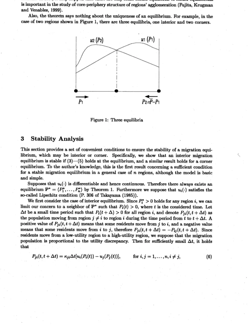
Also, the$\mathrm{t}\mathrm{h}\mathrm{e}\mathrm{o}\mathrm{r}\mathrm{e}\mathrm{m}_{8}\mathrm{a}\mathrm{y}8$ nothing about the $\mathrm{u}\mathrm{n}\mathrm{i}\mathrm{q}\mathrm{u}\mathrm{e}\mathrm{n}\mathrm{e}88$ofanequilibrium. Forexample, inthe
caseof two regions showninFigure 1, there arethree equilibria, one interior andtwo corners.
$\overline{P\uparrow}$ $P\overline{2-\not\simeq-P-}\{$
Figure 1: Threeequilibria
3
Stability
Analysis
This $8\mathrm{e}\mathrm{C}\mathrm{t}\mathrm{i}\mathrm{o}\mathrm{n}$ providesasetofconvenientconditions to ensure
thestabilityofamigration
equi-librium, which may be interior or corner. Specifically, we show that an interior migration
equilibrium$\mathrm{i}8$ stableif (3)$-(5)$ holdsat theequilibrium, and asimilarresult holds foracorner
equilibrium. To the author’s knowledge, thisis the first result concerning a sufficientcondition
for a stable migration equilibriumin a general case of $n$ regions, although the model is basic
and$8\mathrm{i}\mathrm{m}\mathrm{p}\mathrm{l}\mathrm{e}$
.
$\mathrm{S}\mathrm{u}\mathrm{p}\mathrm{p}\mathrm{o}8\mathrm{e}8$that $u_{i}(\cdot)$ isdifferentiableand hencecontinuous. Thereforethere always existsan
equilibrium$\mathrm{p}*=(P_{1}^{*},$
$\ldots$,$P_{n}^{*}\rangle$ by Theorem 1. Furthermore we suppose that $u_{\dot{l}}(\cdot)$ satisfies the
so-called Lipschitz condition (P. 306 of Ihkayama (1985)).
We first cbnsider thecaseofinteriorequilibrium. Since$P_{i}^{*}>0\mathrm{h}\mathrm{o}\mathrm{l}\mathrm{d}8$forany region$i$, wecan
limit our concern to a neighborof$\mathrm{p}*$ such that $P_{i}(t)>0$, where $t$isthe $\mathrm{c}\mathrm{o}\mathrm{n}8\mathrm{i}\mathrm{d}\mathrm{e}\mathrm{r}\mathrm{e}\mathrm{d}$ time. Let
$\Delta t$ bea $8\mathrm{m}\mathrm{a}\mathrm{U}$time period suchthat
$p_{i}(t+\Delta)>0$ for all region$i$, and denote$P_{ji}(t,t+\Delta t)$as
thepopulationmoving from region$j\neq l$ to region$i$during the timeperiodfrom$t$to $t+\Delta t$
.
A$\mathrm{p}\mathrm{o}8\mathrm{i}\mathrm{t}\mathrm{i}\mathrm{v}\mathrm{e}$valueof
$P_{ji}(t,t+\Delta t)$meansthatsome residentsmovefrom$j$to$i$, anda negative value
means that some residents move from$i$ to $j$, therefore $P_{j:}(t,t+\Delta t)=-P_{ij}(t, t+\Delta t)$
.
Since$\mathrm{r}\mathrm{e}\mathrm{s}\mathrm{i}\mathrm{d}\mathrm{e}\mathrm{n}\mathrm{t}_{8}$ movefrom alow-utility region toa
high-utility region, we supposethat themigration
population $\mathrm{i}_{8}$ proportional to the utility discrepancy. Then for sufficiently small $\Delta t$, it holds
that
where $\kappa_{ji}$ is the so-callal speed ofadjustment (Metzler, 1945), which
measures
the speed withwhich residents migrate between regions $i$ and $j$ corresponding to a given utility discrepancy
between regions $i$ and $j$
.
Since $P_{ji}(t,t+\Delta t)=-P_{\dot{e}j}(t,t+\Delta t)$,
it holds that$\kappa_{ji}=\kappa_{\dot{e}j}$
.
Sinceall thefeatures of a region is included in its utility function and all residents arehomogeneous,
residents’ decisions to migrate only dependontheutility$\mathrm{d}\mathrm{i}\dot{\mathrm{s}}\mathrm{c}\mathrm{r}\mathrm{e}\mathrm{p}\mathrm{m}\mathrm{c}\mathrm{y}$
.
Therefore, independent ofthenamesof regions, residents in region$i$ respond to theutihitydiscrepancyofanyother region
with thesame speed of adjustment. That is $\kappa_{ij_{1}}=\kappa_{\dot{\iota}\dot{p}}$ for $\mathrm{a}\mathrm{U}j_{1},j_{2}\neq i$
.
Therefore, $\kappa_{ij}=\kappa$ for all$i$ and $j\neq i$.
We can simply nomalize residents’ utihity function so that $\kappa=1$.
So in thefollowing arguments, we alwayslet $\dot{\kappa}_{ij}=1$
.
For convenience, define $P_{\dot{\iota}i}(t,t+\Delta t)=0$forany $i,$ $t$ and $\Delta t$
.
Then (6) holds forall$i$ and$j$.
Hence
$P_{i}(t+ \Delta t)=P_{i}(t)+\sum_{j=1}^{n}P_{j}i(t,t+\Delta t)=P_{i}(t)+\Delta t\sum_{j=1}[u_{i}(Pi(t))-uj(Pj(t))]n$,
and
$\frac{dP_{i}(t)}{dt}=\lim_{\Delta tarrow 0}\frac{P_{i}(t+\Delta t)-P_{i}(t)}{\Delta t}=\sum_{1\mathrm{j}=}^{n}[u_{i}(Pi(t))-u_{j}(Pj(t))]$,
which leads to dynamics (2). Since we have supposed that $u_{i}(\cdot)$ is differentiable and satisfies
the Lipschitz condition, by extending the domain of definition of$u_{i}(\cdot)$ from $[0,\overline{P}]$ to $(-\infty, \infty)$
suitably, we know that there is a unique and continuous solution of (2) with any initial value
around $\mathrm{p}*$ (Theorem 3.$\mathrm{B}.1$ and itsRemarks of Takayama (1985)).
Summingup all the equations of (2), we find $\sum_{i=1}^{n}dP_{i}(t)/dt=0$, which is consistent with
thefact that $\sum_{=1}^{n}P_{i}(t\rangle$ $=\overline{P}$is aconstant. Therefore we can revise (2) as $\mathrm{f}\mathrm{o}\mathbb{I}\mathrm{o}\mathrm{w}\mathrm{S}$
.
$\frac{dP_{i}}{dt}=(n-1)u_{i}(P\dot{\iota})-j-1\sum_{j\overline{\neq}i}^{\mathfrak{n}-1}u_{j}(P_{j})-u_{n}(\overline{P}-n-j=1\sum P_{j})1$, $i=1,$
$...\cdot,n-1$
, (7)
Following Tabuchi (1986), we denote $\mu:=u_{i}’(P_{i^{*}})$ and denote the characteristic polynomial of
matrix$A$ as $\Psi_{A}(\lambda)=\det[A(\lambda)]$, where$A=[a_{ij}]_{\mathrm{t}^{n}}-1)\mathrm{x}\mathrm{t}^{n-}1)’ A(\lambda)=[a(\lambda)_{i}j]_{\mathrm{t}n-}1)\mathrm{X}(n-1)$ ’ and
$a_{ij}=\{$
$(n-1)\mu_{i}+\mu_{n}$, fori $=j$
$-\mu_{j}+\mu_{n}$, for $i\neq j$ ’
(8)
$a(\lambda)_{\dot{\iota}j}=\{$
$(n-1)\mu_{\dot{l}}+\mu_{n}-\lambda$, for $i=j$ $-\mu_{j}+\mu_{n}$, $\mathrm{f}\mathrm{o}\mathrm{r}i\neq j$
After renamin$\mathrm{g}$ the regions if necessary, we suppose that$\mu_{1}\geq\mu_{2}\geq\ldots\geq\mu_{n}$
.
There are $n-1$roots (possiblymultiple) of the characteristic equation $\Psi_{A}(\lambda)=0$, which are$\mathrm{c}\mathrm{a}\mathrm{U}\alpha 1$eigenvalues.
It is knownthat equilibrium $\mathrm{p}*$ of$\langle$7) is stable if all the Ieal partsof the eigenvalues of $A$ are
negative (Gantmacher, 1960), and is unstable if there is at least
one
eigenvalue is with positivereal part. We can show that $\mathrm{g}$ theeigenvalues of $A$ are realnumbers, which are all negative
if and only if(3)$-(5)$ hold. Rrthermore, from Tabuchi (1986), weknow that if (3) is violated
then there is at leastonepositiveeigenvalue and the dynamics is unstable. Therefore, weaffirm
Theorem 2 An interiorequilibrium isstable
if
(3)$-(5)$ hold at the equilibriumjif
(3) is violated,Remark Wecan further show that if (3) holds but (4)or (5)is violated, then $0$is
an
eigenvalueof$A$
.
Since the differentialequationtheory doesnot completely disclose thecriticalcasewith azeroeigenvalue,
we
arenotsurewhether the dynamics is stableorunstable in thiscase. However,almost $\mathrm{a}\mathrm{U}$economics researches (Okabe, 1980; Nakajima, 1995) omit the discussionof this case
and think that having a zero eigenvalue implies that the dynamics is unstable. In this sense,
(3)$-(5)$ become necessaryand sufficient conditions for the stability.
Next we turn to thecaseofcornerequihibrium. In migration study, itisreasonabletosuppose
that the inequalityin (1) holds
strictly1.
That is,$u^{*}>u_{j}(0\rangle$ for all$j$ such that $P_{j}^{*}=0$
.
(9)By (1) and (9), we can renamethe regions so that
$\{$
$P_{i}^{*}\neq 0$ and $u_{i}(P_{i^{*}})=u^{*}$, for$i=1,$
$\ldots,$$n_{1}$;
$P_{j}^{*}=0$ and $u_{\mathrm{j}}(0)<u^{*}$, for$j=n_{1}+1,$$\ldots$
,
$n$; $u_{1}’(P_{1^{*}})\geq\cdots\geq ui(\prime P_{i}*)\geq\cdots\geq u_{\mathrm{b}}’(1P^{*})n1^{\cdot}$(10)
Consider an initial population distribution $\mathrm{P}(t)=\langle P_{1(t),\ldots,P_{n}(t\rangle}\rangle$
.
If$P_{\mathrm{j}}(t)=0$, then nonemoves from region $j$ to other regions but some residents may migrateinto region $j$
.
Therefore(6) shouldbe revised as follows
$P_{J^{i}}’(t,t+\Delta t)=\{$
$\Delta t[u_{i}(Pi(t))-uj(P_{j}(t))1$, if$P_{i}(t)>0,P_{j}(t\rangle>0$, $\Delta t\min\{0,u_{i(}Pi(t))-u\mathrm{j}(P_{j}(t))\}$, if$P_{i}(t)>0,P_{j}(t)=0$,
$\Delta t\max\{0,u_{i}(P_{i(t)})-uj(P_{j}(t))\}$, if$P.(t)=0,P_{j}(t)>0$,
$0$, if$P_{i}(t)=P_{j}(t)=0$
.
Hence the dynamics for a
corner
equilibrium takes the$\dot{\mathrm{f}}\mathrm{o}$llowing form: for $\mathrm{i}=1,$
$\ldots,$ $\mathrm{n}$
,
$\frac{dP_{i}(t)}{dt}=\{$ $j=1, \ldots,n\mathrm{I}P_{\tilde{g}}\mathrm{t}\sum_{0t)>}[u_{i(P_{i}}(t))-uj(Pj(t))]$ if$P_{i}(t)>0$, $+ \sum_{0j=1,\ldots,n|P_{j}\mathrm{t}^{t})=}\min\{0,ui(Pi(t))-u_{\mathrm{j}}(Pj(t))\}$,
$j=1, \ldots,n|P_{j}(\sum_{t)>0}\max,\mathrm{t}0,u\dot{*}(P_{i}(t))-u_{j}(Pj(t))\}$, if$P_{i}(t)=0$.
(11)Note that the aboveequationsimply that $\sum_{i=1}^{n}dP_{i}(t)/dt=0$ for all$t$, which isconsistent with
the assumption ofconstant popuhtion$\overline{P}$
.
Remember that $u_{i}(\cdot)$satisfies the Lipschitz condition,byextendingthedomainofdefinition
of$u_{i}(\cdot)$ from $[0,\overline{P}]$ to $(-\infty, \infty)$ suitably, weknow that there is a unique and continuous solution
of (11) with any initial condition around $\mathrm{p}*$
.
Our stabihty conclusion for acorner equilibriumis stated in the $\mathrm{f}\mathrm{o}\mathbb{I}\mathrm{o}\mathrm{W}\dot{\mathrm{m}}\mathrm{g}$ theorem. The result is also very intuitive. Starting from initial
distribution around $\mathrm{p}*$, the residents in regions
$n_{1}+1,$$\ldots,n$ will migrate to regions 1,...,$n_{1}$
because the utihties in Iegions $n_{1}+1,$$\ldots,n$ are lower. Conditions (12) $-(14)$ are similar to
(3)$-(5)$, whichensure that thepopulation distribution ($P_{1}^{*},$$\ldots,P_{\mathrm{n}_{1}}^{*}\rangle$ will be stableif thereare only $n_{1}$ regions totally.
1 An equihbriummay be either stable or unstable if$u^{*}=u_{\overline{\mathrm{J}}}(\mathrm{o})$ instead of(9) $\mathrm{h}\mathrm{o}\mathrm{l}\mathrm{d}8$ for a region $j$
.
Themathematical$\mathrm{a}\mathrm{n}\mathrm{a}\mathrm{l}\mathrm{y}8\mathrm{i}8$for$\mathrm{t}\mathrm{h}\mathrm{i}8$caseisverytroublesome and thiscase seemsto be unhkely inammigration eqmilibrium
of real$\mathbb{R}$
.
Therefore almost$\mathrm{a}\mathrm{U}$economics researchers (for example, Rjita, Krugnan and Veneables, 1999) omit the diseussion of thiscase,evenwhen$n=2$
.
Theorem 3
If
$n_{1}=1$, then equiliffium$\mathrm{p}*=\mathrm{t}P_{1}^{*},$ $\ldots,P_{n}^{*}$) satishing (10) is always stable.If
$n_{1}\geq 2$, then equihbrium $\mathrm{p}*sabf\dot{w}ng(10)$ is stable
if
$(n_{1}-1)u_{1}(\prime P_{1^{*}})+u_{\dot{l}}’(P_{i^{*}})\leq 0$, $\forall i=2,$$\ldots,n_{1}$
,
(12)the inequality
of
(12) hous $Sm_{ctly}$for
at leastone
$i=2,$$\ldots,n_{1}$, (13)if
$u_{1}’(P_{1^{*}})=0$, then $u_{2}’(P_{2^{*}})<0$.
(14)If
(12) is niolated, then$\mathrm{p}*$ is unstable.Similar to the remark after $\mathrm{T}\mathrm{h}\infty \mathrm{r}\mathrm{e}\mathrm{m}2$, ifwe treat the critical case ofzero eigenvalue as
unstable, then (12)$-(14)$ becomenecessary and sufficientconditions.
RomTheorems2 and 3, weknow that in thecaseofFigure 1, twocornerequilibriaarestable
and the interior oneis not. Althoug Theorem 1 ensuresthat at least oneequilibrium, it does
not ensure the existence ofa stable equihibrium. In thecase that $n=2,$ $u_{1}(P_{1})=u_{2}(\overline{P}-P_{1})$
,
each residentialdistribution forms an equilibrium butnone is (asymptoticffiy) stable.
4 Conclusions
This paper investigates a deterministic migration model among $n$ regions in the case ofzero
natural growth. First, it is shown that thecontinuity of residents’ utility functionsensures the
existence of a migration equilibrium. Then sufficient conditions are given for the stability of
such an equilibrium.
Although the modelused in thispaperis basicandsimple,but the discussion here is rigorous.
To the author’s knowledge, no other paper shows the existence of a migration equilibrium
explicitly andnonehasgivenany sufficientconditionforthestabihityofa migrationequilibrium
in the case of$n$ regions before.
It is known that the recent economic geography literature is strongly related to stability
analysis ofa migrationequilibrium, the results of this paper is expected to beapplicable in the
research ofeconomic geography.
Finally,theresultsof thispaperarevaluabletobe$\mathrm{e}\mathrm{x}\mathrm{t}\mathrm{e}\mathrm{n}\mathrm{d}\mathrm{e}\mathrm{d}$
’
tosome more realisticandmore
complex models. First, ourresults depend stronglyon the assumption that the utility function
$u:(P_{\dot{l}})$ is only related to the population size of region $i$
.
A general function may be related tothe populationsizes of otherregions. Thestabihityconditionsderived in this paperdonot hold
in this general $\mathrm{m}o\mathrm{d}\mathrm{e}\mathrm{L}$ Second, our model is deterministic but there are many good stochastic
models (Tabuchi, 1986; Weidlich and Haag, 1988; O’Connel, 1997). The stabihity research on
somestochastic models mayreveal more$i\mathrm{m}\mathrm{p}_{\mathrm{o}\mathrm{r}\mathrm{t}\mathrm{n}}\mathrm{a}\mathrm{t}\backslash$facts.
A&nowledgement: Theauthorthanks T. Tabuchi of The University of Tokyo, Y. Yamamura
and H. Takatsuka ofKagawa Univerisity and twoanonymous referees for beneficial discussions
and comments.
References
Berglas E., 1984. Quantities, qualities and multiple public services in the Tiebout modeL
Journal ofPublicEconomics 25, 299321.
Bewley T. F., 1981. A critique of Tiebout’s$\mathrm{t}\mathrm{h}\infty \mathrm{r}\mathrm{y}$
. oflocal public expenditures. Econometrica
Boadway R. W. and F. R. Flatters, 1982. Efficiency and equalization payments in a $\mathrm{f}\alpha \mathrm{l}\mathrm{e}\mathrm{r}\mathrm{a}‘ 1$
system of govemment: A synthesis and extension of recent results. Canadian Journal of
Economics 15, 613-633.
Fujita M., P. Krugman and A. J. Veneables, 1999. The SpatialEconomy Cities Regions and
*
International Rade,The MIT Press.
Gantmacher R. R., 1960. TheTheoryof Matrices, Volume 2, Chelsea, New York.
Konishi H., 1996. Voting with ballots and feet: existence ofequilibrium in a local public good
economy. Journal of Economic $\mathrm{T}\mathrm{h}\infty \mathrm{r}\mathrm{y}68$, 480-509.
Krugman P., 1991. Increasing returns and economic geography. Journal of PoliticalEconomy
99, 483499.
Metzler L. A., 1945. Stability of multiple markets: the Hicks conditions. Econometrica 13,
. 277-292.
NakajimaT., 1995. Equilibrium with an umderpopulated region and anoverpopulated region.
Regional Scienceand Urban Economics 25, 109-123.
Nechyba T. J.,
1997.
Existence of equilibrium and stratification in local and hierarchicalTiebout economies with property taxes and voting. Economic Theory 10, 277-304.
O’Connell P. G. J., 1997. Migration under uncertainty: “By your luck” or “Wait and see”.
Journal ofRegional Science 37, 331-347.
Okabe A., 1980. Stable state conditions of population-dependent migration models under a
zero natural growth rate. Journal of RegionalScience 20, 353-364.
Tabuchi T., 1986. $\dot{\mathrm{E}}\mathrm{x}\mathrm{i}\mathrm{s}\mathrm{t}\mathrm{e}\mathrm{n}\mathrm{c}\mathrm{e}$
and stabihity of city-size distribution in the gravity and logit
models. Environment and PlanningA 18,
1375-1389.
Takayama A.; 1985. Mathematical Economics, Cambridge University Press.
Weibull J. W., 1995. Evolutonary GameTheory, The MIT Press.
Weidlich A. and H. Haag, $\mathrm{e}\mathrm{d}\mathrm{s}.$, 1988. InterIegional Migration, Dynamic
$\mathrm{T}\mathrm{h}\infty \mathrm{r}\mathrm{y}$and