i.i.d.カオス系列を用いたストリーム暗号システム (確率数値解析に於ける諸問題, V)

Stream

Cipher Systems

Using aChaotic

Sequence of

I.I.D

Random

Variables

i.i.d.

カオス系列を用いたストリーム暗号システム

Tohru

KOHDA

香田徹 e-mail: [email protected]

Department of Computer

Science

and

Communication

Engineering,

Kyushu University,

Hakozaki 6-10-1, Higashi-ku, Fukuoka, 812-8581, Japan

九州大学大学院システム情報科学研究院情報工学部門

〒

812-8581

_{福岡市東区箱崎6 丁目 10-1}

Abstract- Asequence of i.i.d. binary random variables has found significant

applica-tions in modern digital communication systems, such

as

aspreading spectrum sequence for

a

DS/CDMA system and akey-stream sequence for astream cipher system. In this paper,

after reviewing the generation method ofsequences of i.i.d. binary random variables

gener-ated by chaotic dynamics

we

give astream cipher system using asequence of i.i.d. binary

randomvariables which has cryptographic resistance for severalkinds of cryptanalysis based

on

correlation functions.

$\mathrm{K}\mathrm{e}\mathrm{y}\mathrm{w}\mathrm{o}\mathrm{r}\mathrm{d}_{\mathrm{S}}-\mathrm{s}\mathrm{t}\mathrm{r}\mathrm{e}\mathrm{a}\mathrm{m}$cipher, keystreamsequences, randomsequence,

i.i.d.

sequence,

chaotic

dynamics, Cryptanalysis, aut0-/cross-correlation function, secret key

1Introduction

Asequence of independent and identicallydistributed $(i.i.d.)$ binary random variables $[1]-[4]$

hasfoundsignificant applicationsin moderndigitalcommunication systems such

as

in spread

spectrum (SS) communicationsystems [5]

or

cryptosystems $[6, 7]$

as

well

as

in computational

applications requiring random numbers $[8, 9]$

.

Such abinary sequence

can

be generated

in various ways. _{Nevertheless, linear feedback shift register} (LFSR) sequences which have

already been thoroughly investigated based

on

finite field theory

are

employed in nearly aU

the methods [10].

It is, however, $\mathrm{w}\mathrm{e}\mathrm{u}$ knownfromprobability theory $[1]-[3]$

and ergodic theory [4] that coin

tossing is atheoretic model that generates

asequence

of i.i.d. binary random variables in

the following

sense.

Imagine $n$ independent tosses of afair coin. If

we

label 1and 0instead

of head and tail, then the resulting binary

sequence

of length $n$ gives uniquely both the

associated dyadically rational number and

one

of2’$l$

disjoint half-0pen subintervals of widt$\mathrm{h}$

数理解析研究所講究録 1240 巻 2001 年 74-87

$d,(\omega)$

$d_{2}\mathrm{t}\omega)$

$d_{\mathrm{J}}(01)$

Figure 1: Binary functions $d_{k}(\omega)$ which define Rademacher functions $rk(\omega)$

.

$2^{-n}$ whose left endpoint is the dyadically rational number.

On

the other hand, choose

a

dyadically rational number $\omega$ at random and consider the ‘map’ (or ‘transformation’) on the

half-0pen unit interval $[0, 1)$, defined by $\tau(\omega)=2\omega$(modl), referred to

as

the dyadic map.

Then the dyadic map shifts the digit

one

place to the left ofthe binary expansion of$\omega$

.

In

such

an

expansion, the binary function is sometimes referred to

as

the

Rademacher

_function.

Thus throwing adie may be

seen as

both adeterministic and arandom event.

Ulam andvonNeumann [11] pointed out the logisticmap, themost famous chaotic one, is

agoodcandidateof pseudorandomnumbergenerators. Ontheotherhand,several encryption

algorithms based

on

chaos theory [12]-[18] have been discussed (see, for example, thesurvey

in [18]$)$

.

We have recently givenseveral methodsforgenerating abinarysequencebased

on

chaotic

dynamics [19]-[21] and asimplesufficient conditionfor

some

classofergodicmapsto produce

asequence of i.i.d. binary random variables $[23, 24]$. Furthermore,

we

have proposed

a

cryptosystem in afloating point environment whose keystream sequences

are

chaotic bit

sequences $[25, 26]$

.

In this paper, wefirst review asufficient condition $[23, 24]$ for

some

class of ergodic maps

and theirassociatedbinary functions to produceasequence ofi.i.d. binaryrandomvariables.

Seconddly,

we

give astream cipher system whose running key is asequence of i.i.d binary

random variables and show such asystem has its cryptographical strength $[25, 26]$

.

2Design of

Binary Sequences Using

PM

Maps

2.1

Sequences

Generated

by

Bernoulli

Shift and

Rademacher Function

Let

us

start byreviewing fundamentalsubjects from the textbooks ofelementary probability

theory $[1]-[3]$ and ergodic theory [4].

Let $\omega$ be apoint drawn at random from the half-0pen unit interval $[0, 1)$

.

With each

$\omega$

associate its nonterminating binary expansion

$\omega=\sum_{k=1}^{\infty}\frac{d_{k}(\omega)}{2^{k}}=0.d_{1}(\omega)d_{2}(\omega)\cdots$, wwhhoesree$d_{i}(\omega)\in\{0,1\}$

.

(1)

Imagine

now

acoinwithfaces labeled 1and

0instead

ofthe usual heads (H) and tails (T). If

$\omega$ is drawn at random, $\{d_{k}(\omega)\}_{k=1}^{\infty}$ behaves

as

if it resultedfrom

an

infinite sequence oftosses

ofafair coin On the other hand, define the map $\tau_{B}(\cdot)$, referred to

as

the Bernoulli

shift

or

dyadic map by $\tau_{B}(\omega)=2\omega$, $\mathrm{m}\mathrm{o}\mathrm{d} 1$ which gives $\tau_{B}(\omega)=0.d_{2}(\omega)d_{3}(\omega)\cdots$

.

This implies that

$\tau_{B}(\cdot)$

shifts the

digits

one

place to the left, namely, $d_{k}(\tau_{B}(\omega))=d_{k+1}(\omega)$,

for

$k\geq 1$

.

The

75

$T=\{t_{0}|$

$T=\{t_{l}$

.

t,.-t,$|$

$T=\mathrm{I}\mathrm{t}d=t_{\phi}t.t.t- l,e=\mathrm{J})- i,l- t_{2’}’\sim 2Ji_{1}$,

Figure 2: Independentpulse

functions

defined by $C_{T}(\omega)$

.

functions

$d_{k}(\omega)$,$k=1,2$,$\cdots$

are

often replaced by the

Rademacher

fienctions

$[1, 3]$ _defined

as, $rk()=1-2dk(\omega)$, $k=1,2$,$\cdots$

.

Since

the

functions

$r_{k}(\omega)$, $k=1,2$,$\cdots$ furnish

us

with

amodel_{of independent tosses of a“fair” coin, their values give rise to “independent random}

variables”. Figure 1shows the binary

functions

$d_{k}(\omega)$

.

2.2

Binary Sequences

Generated

by

Ergodic Maps

In the application of chaotic dynamics to cryptosystem, the dyadic map is impracticable with

the help ofacomputer with its limited accuracy in the

sense

that the period of its chaotic

orbit is very short. Ofcruicial importance is the question whether any other maps than the

dyadic map

can

realizecoin tossing

or

not.

Let

us

start withgiving threesimple methods [19]-[21] forobtainingbinarysequences ffom

chaotic real-valued sequences $\{\omega_{n}\}_{n=0}^{\infty}$, generated by

an

ergodic

map

_{$\tau(\cdot):J=[d, e]arrow J$}

$\omega_{n+1}=\tau(\omega_{n})$, $\omega_{n}=\tau^{n}(\omega_{0})\in J$,

n

_$=1,$2,_{\cdots .} (2)

Method-l: Define athreshold function $\Theta_{t}(\omega)$

as

Qt(w) _$=\{$

mentary

function

$\overline{\Theta}_{t}(\omega)=1-\Theta_{t}(\omega)$

.

0for $\omega<t$,

and its

comple-1for $\omega$ $\geq t$

Method- 1: For $\omega(|\omega|\leq 1)$ introduce its binary representationof.$\cdot$

$|\omega|=0.A_{1}(\omega)A_{2}(\omega)\cdots A:(\omega)\cdots$,$A_{:}(\omega)\in$

{0,1}

(3)

where

$A_{i}( \omega)=\bigoplus_{r=1}^{2}.\{\Theta_{-\frac{r}{2}}$

.

$( \omega)\oplus\Theta_{\frac{r}{2}}.(\omega)\}=\sum_{r=1}^{2}.(-1)^{r-1}\{\Theta_{\frac{r}{2}}.(\omega)+\overline{\Theta}_{-\frac{r}{2}}.(\omega)\}$, (4)

and $\oplus \mathrm{d}\mathrm{e}\mathrm{n}\mathrm{o}\mathrm{t}\mathrm{e}\mathrm{s}$ modulo 2addition.

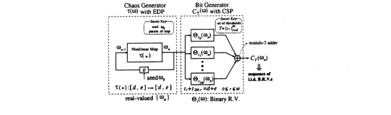
Method-S: [23] Define abinary function with the set of thresholds, T$=\{t_{r}\}_{r=0}^{M_{T}}$, definedby

$C_{T}( \omega)=\oplus\ominus_{t_{r}}(\backslash \omega)=\sum_{rr=0=0}^{M_{T}}(-1)^{r}\Theta_{t_{r}}(\omega)M_{T}$, (5)

then

we

get the following examples:

Example 1:

_Ct{w)

$=\mathrm{Q}\mathrm{t}$ (w) when $M_{T}=0$

.

$(’)-d$

Example $\mathit{2}\ovalbox{\tt\small REJECT}$ The value of C [0,1] has

e-d

$\frac{\omega-d}{e-d}=0.B_{1}(\omega)B_{2}(\omega)\cdots B_{i}(\omega)\cdots$ , where$B_{i}(\omega)\in\{0,1\}$ (6)

which implies that $\mathrm{C}\mathrm{T}(\mathrm{u})=\mathrm{B}\mathrm{i}\{\mathrm{u}$), when$M_{T}=2^{i-1}$,$t_{r}=(e-d) \frac{r}{2}$

.

$+d$

.

If the interval

$J=[0,1]$, then $A_{:}(\omega)=B_{i}(\omega)$

.

The binary function

Ct{w)

is referred to

as

the binary pulse

function. Figure 2shows its examples. Note that $\mathrm{B}\{(\mathrm{u})=d_{i}(\omega)$ when $\tau(\cdot)=\tau_{B}(\cdot)$

.

2.3

The Equidistributivity

Property

EDP and the Constant

Summation

Property

CSP

It is

an

important problem whether any other maps and their

associated

binary functions

than the dyadic map and the Rademacher function, respectively

can

realize

asequence

of

i.i.d. binary random variables

or

not. Recently

we

have replied in the affirmative: There is a

wide class ofergodic maps with the equidistributivity property (EDP) and their associative

binary functions with the constant summation property (CSP) $[23, 24]$

.

To review this,

we

begin bydefining the class ofmapsto bediscussed and introducingseveral definitions needed

in this discussion.

Define apiecewise monotonic (PM) onto ergodic map $\tau(\cdot)$ : $J=[d, e]arrow J$ that satisfies

the following conditions:

i) there is apartition $d=d_{0}<\cdots<d_{N_{\mathrm{r}}}=e$ of $J$ such that for each integer $i=$

$1$,$\cdots$ ,$N_{\tau}$, $(N_{\tau}\geq 2)$ the restriction of $\tau(\cdot)$ to the interval $J_{i}=[d_{i-1}, d_{\dot{l}})$, denoted by

Bi{

$\mathrm{u})$, is

a

$C^{2}$ function;

as

well

as

ii) $\tau(J_{i})=(d,$e);

iii) $\tau$ has aunique ACI measure, denoted by $f^{*}(\omega)d\omega$

.

Definition 1For$PM$onto rnap with its $ACI$measure, the partition $\{J_{i}\}_{i=1}^{N_{\tau}}$ is

referred

to

as

the trivial partition

of

the interval $J$

.

Definition 2 $[\mathit{2}7, 28]$ The Perron-Frobenius operator (or

‘transfer’

operator) $P_{\tau}$ acting on

the

_{function of}

bounded variation $\mathrm{H}(\mathrm{w})\in L^{\infty}$

for

$\tau(\omega)$ is

defined

as

$P_{\tau}H( \omega)=\frac{d}{d\omega}\int_{\tau^{-1}([d,\omega}H(\gamma_{)})dy=\sum_{j=1}^{N_{\tau}}|g_{/}’.(\omega)|H(g_{i}(\omega))$ , (7)

where

Ct{w)

$=\tau_{i}^{-1}(\omega)$ is the $i$-th preimage

of

$\omega$.

This implies $P_{\tau}$ is the (discrete-time) evolutionoperator ofthe probability density function

under the map$\mathrm{r}()[27]$

.

Note that the

ACI

measure

$f^{*}(\omega)d\omega$ satisfiies the invariant equation

$P_{\tau}f^{*}(\omega)=\mathrm{C}\mathrm{t}\{\mathrm{w}$), referred to

as

the P-F equation.

Definition 3 [23] The rnap is said to satisfy equidistributivityproperty (EDP)

if

the relation

$|g’, \cdot(\omega)|f^{*}(g_{\dot{l}}(\omega))=\frac{f^{*}(\omega)}{N_{\tau}}$, $1\leq i\leq N_{\tau}$ (8)

Definition 4[23]

_{If for}

a class

_of

maps with EDP its associated

_function

$F(\cdot)$

satisfies

$\frac{1}{N_{\tau}}\sum_{\dot{l}=1}^{N_{\tau}}F(g_{i}(\omega))=\mathrm{E}[F]$,

(9)

then$\mathrm{F}(-)$ is said to satisfy the constant summationproperty (CSP), where

$\mathrm{E}[F]$, theensemble

average

_of

$F(\omega)$, is

defined

in

Definition

8.

Remark 1

_f23J

Consider a

random variable$\mathrm{F}(\mathrm{u})$ and its weightedrandom

function

$F(\omega)f^{*}(\omega)$

with the weight

_function

$f^{*}(\omega)$

.

Observe

$P_{\tau} \{F(\omega)f^{*}(\omega)\}=\frac{1}{N_{\tau}}\sum_{\dot{l}=1}^{N_{\mathrm{r}}}|g_{\dot{l}}’(\omega)|f^{*}(g:(\omega))F(g:(\omega))$

.

(10)

An easy consequence

_of

the

_definition

is that

_if

given

a

weighteddensity

_function

with respect

to

a

random variable $\mathrm{F}(\mathrm{u})$ with _{$\mathrm{E}[F]\neq 0$},

defined

by $F(\omega)f^{*}(\omega)$, both

of

the _$CSP$

of

$F(\omega)$

and the $EDP$

of

$f^{*}(\omega)$

are

satisfied, then $\frac{F(\omega)}{\mathrm{E}[F]}f^{*}(\omega)$ is

an

invariant

function

under the map

$\tau(\cdot)$

.

Definition 5(Topological Conjugation)$[28, \mathit{3}\mathit{1}]$ Two

transformations

$\overline{\tau}$: $\overline{I}arrow\overline{I}$ and

$\tau$ : $Iarrow$

I on intervals $\overline{I}$

and I are called topological conjugate

_if

there exists a homeomorphism $h$:

$\overline{I}\frac{\mathrm{o}\mathrm{n}\mathrm{t}\mathrm{q}}{}$

, $I_{f}$ such that $\tau(\omega)=h\mathrm{o}\overline{\tau}\mathrm{o}h^{-1}(\omega)$

.

Suppose $\tau(\cdot)$ and $\overline{\tau}(\cdot)$ have their ACI

measures

and

denote them by $f^{*}(\omega)d\omega$ and $\neg f(\overline{\omega})\Phi$,

respectively. Then, under the topological conjugation, these ACI

measures

have the relation

$f^{*}( \omega)=|\frac{dh^{-1}(\omega)}{d\omega}|f(h^{-1}(\omega))\neg$

.

(11)

It is easily checked ffom simple calculation that the EDP is invariant under the topological

conjugation.

Examples ofthe mapswith theirACI

measures

which satisfy theEDP

are

listed

as

follows.

(1) $R$-adic map _{$(N_{\tau}=R, R=2,3,4, \cdots)$}

$\tau_{R}(\omega)=R\omega$ $\mathrm{m}\mathrm{o}\mathrm{d} 1$, $\omega$ $\in[0,1]$, $f^{*}(\omega)d\omega$$=d\omega$,

(2) logistic map $(N_{\tau}=2)[11]$

$L_{2}(\omega)=4\omega(1-\omega),\omega$ _$\in[0,1]$, $f^{*}( \omega)\mathrm{d}v=\frac{d\omega}{\pi\sqrt{\omega(1-\omega)}}$,

(3) Chebyshev map ofdegree$p(N_{\tau}=p, p=2,3,4, \cdots)$ $[29]-[31]$

Tp{u) $=\cos(p\cos^{-1}\omega)$, $\omega$ $\in[-1,1]$, $f^{*}( \omega)d\omega=\frac{d\omega}{\pi\sqrt{1-\omega^{2}}}$,

(4) Zigzag map withp branches $(N_{\tau}=p,$p$=2,$3,4,

\cdots )

[31]

$N_{p}(\omega)=(-1)^{\Psi^{v\rfloor}}p\omega$, $\omega$ $\in[0,$ 1], $f^{*}(\omega)d\omega=M$,

Figure 3: Sequence generator of$\mathrm{i}.\mathrm{i}.\mathrm{d}$

.

binary random variables for astream cipher system

using chaotic dynamics.

where $\lfloor x\rfloor$ denotes the largest integer not greater than $x$ and $N_{2}(\omega)$ is referred to

as

the tent

map.

Ulam and von Neumann [11] pointed out that the logistic map $L_{2}(\omega)$ and the tent map

$N_{2}(\overline{\omega})$

are

topological conjugate via

$h^{-1}(\omega)=\underline{2}\sin^{-1}\sqrt{\omega}$

. On

the other hand, Grossmann

andThomae [31] observed that$T_{p}(\omega)$ and

$N_{p}(\overline{\omega})^{\pi}\mathrm{a}\mathrm{r}\mathrm{e}$

topological conjugate via$h(\overline{\omega})=\cos\pi\overline{\omega}$

.

Now let

us

consider astationary real-valued sequences $\{F(\omega_{n})\}_{n=0}^{\infty}$, where $\omega_{n}=\tau^{n}(\omega_{0})$

.

Definition 6(Birchoffindividual ergodic theorem)$[4, 28]$ The time average

of

any $L_{1}$

func-than $\mathrm{F}(-)$ along a chaotic real-valued trajectory $\{\omega_{n}\}_{n=0}^{\infty}$ _$gen$erated by the map (2), denoted

by Averagc4$\{F\}$,

defined

by Average4 $\{F\}--\lim_{Tarrow\infty}\frac{1}{T}\sum_{n=0}^{T-1}\mathrm{F}(\mathrm{u}\mathrm{n})$ is equal almost everyw here to

the expectation

_of

$F(\omega)$,

defined

by $\mathrm{E}[F(X_{n})]=\int_{I}F(X_{n})f^{*}(\omega)d\omega$

.

From the stationarity

of

process,

we

denote $\mathrm{E}[\mathrm{F}\{\mathrm{X}\mathrm{n})\}$ by $\mathrm{E}[F(X)]$

or

simply $\mathrm{E}[F]1$

Ofmajor importance to theinvestigationofstatistical propertiesof twosequences $\{F(\tau^{n}(\omega))\}_{n=0}^{\infty}$

and$\{G(\tau^{n}(\omega))\}_{n=0}^{\infty}$is their$2\mathrm{n}\mathrm{d}$-ordercross-covariancefunction with delay$\ell=0,1$,$\cdots$ which

is defined by

$\rho(\ell;F, G)=\int_{I}(F(\omega)-\mathrm{E}[F])(G(\tau^{\ell}(\omega))-\mathrm{E}[G])f^{*}(\omega)d\omega$, (12)

which denotes the aut0-covariance function when $F=G$

.

Remark 2Note that the opertaor$\mathrm{P}\mathrm{T}(-)$ has the mostimportantproperty

of

the P-F operator

$P_{\tau}$:

$\int_{J}F(\omega)G(\tau(\omega))d\omega$ $= \int_{J}P_{\tau}\{F(\omega)\}G(\omega)d\omega$, (13)

where $G(\tau(\omega))$ in the integrand in the $Ihs$ is

referred

to

as

the Koopman operator,

as

the

adjoint operator

_of

the Perron-Frobenius operator in a Hilbert space $[\mathit{2}\mathit{8}, 32]$

.

Using (13),

we

get the

rew

ritten$form$

of

(12)

$\rho(\ell;F, G)=\int_{I}P_{\tau}^{l}\{F(\omega)f^{*}(\omega)\}G(\omega)d\omega$ $-\mathrm{E}[F]\mathrm{E}[G]$

.

(14)

1 _{It should be noted that expectation} $\mathrm{E}[\cdot]$ is used here in asense applicable to deterministicsequencesof

the form (2), anddiffers from the standardonefor stochasticsequenceswhich will involve ajoint probability

densityfunction

Equation (10) andcondition ii) ofthe onto map $\tau(\cdot)$ give

Lemma 1[23] The $PM$ onto maps $\tau(\cdot)$ with $EDP$ satisfy

$P_{\tau}\{\Theta_{d}\dot{.}(\omega)f^{*}(\omega)\}=\mathrm{E}[\Theta_{d:}]f^{*}(\omega)$

.

(15)

Lemma 2 [23]For

a

class

_of

maps with $EDP$, the following three _{symmetric properties:}

SI: the symmetric binary

_function

$C_{T}(\omega)$,

defined

as

$t_{r}+t_{2M-r}=d+e$,

r

$=0,$ 1,\cdots ,M;

S2: the symmetric

ACI

measure,

_defined

as

$f^{*}(d+e-\omega)=f^{*}(\omega)$;

S3: the symmetric map,

_defined

as

$\tau(d+e-\omega)=\tau(\omega)$, $\omega$ $\in I$

give

$P_{\tau}\{C_{T}(\omega)f^{*}(\omega)\}=\mathrm{E}[C_{T}]f^{*}(\omega)$

.

(16)

Remark 3Relation (16) is a generalized version

_of

(15); the

CSP

_of

$\mathrm{F}(\mathrm{J})$ guarantees their

zero

correlations, $\rho(\ell,$F,$G)=0$,

for

‘positive’ delay$\ell$ irrespective

of

$G(\omega)$

.

Next, let $\mathrm{U}=U_{0}U_{1}\cdots U_{m-1}$ be

an

arbitrary string of $m$ binary digits where $U_{n}\in$

$\{0,1\}(0\leq n\leq m-1)$

.

_{Then there}

are

$2^{m}$ possible strings. Let $\mathrm{u}^{(r)}=u_{0}^{(r)}u_{1}^{(r)}\cdots u_{m-1}^{(r)}$ be

the $r$-th string. Introducing abinary random variable

$\Gamma_{n}(\omega;$F,$\mathrm{u}^{(r)})=F(\omega)u_{n}^{(r)}+\overline{F}(\omega)\overline{u}_{n}^{(r)}$ (17)

for any binary

function

$\mathrm{F}(\mathrm{v})$ with CSP,

we can

get [23]

Theorem 1: The probability

_of

the event$\mathrm{u}^{(r)}$

in

an

_infinite

binary

sequence

$\{C_{T}(\omega_{n})\}_{n=0}^{\infty}$

is given by

$Pr(\mathrm{u}^{(r)}; C_{T})$ $=$ $\int_{I}\{\prod_{n=0}^{m-1}\Gamma_{n}(\omega_{n};C_{T}, \mathrm{u}^{(r)})\}f^{*}(\omega)d\omega$

$=$ $\mathrm{E}[C_{T}]^{s}(1-\mathrm{E}[C_{T}])^{m-s}$, (18)

where$s$ is the number

of

1in $\{u_{n}^{(r)}\}_{n=0}^{m-1}$

.

This implies $\{C_{T}(\tau^{n}(\omega))\}_{n=0}^{\infty}$ is asequenceof i.i.d. binary random variables with probability

$\mathrm{E}[\mathrm{C}\mathrm{t}]-$ Note that

we

can

get afair Bernouli sequence when _{$E[Cr]= \frac{1}{2}$}, that is,

an

m-distributed binary randomsequence. Figure 2shows

an

example of symmetric binaryfunction

$C_{T}(\omega)$

.

3Stream

Cipher System

3.1

Stream

Cipher System

Using

Chaotic Dynamics

We employ the s0-called binary additive stream ciphers in which ashort secret key $\vec{K}=$

$(s_{1}.s_{2},$_{\cdots ,$s\#)$} is used only to controlakeystream generator. We havesecret key parameter

$4$

,

0 $,*$ $\mathrm{r}$ $\infty$ $*$ $u$ $*$ 00 ,0 , $\infty$ $u$ $\infty$ $\infty$ 90 $\prime l$ $\infty$ , $*$ $\infty$

.

Time Delay ’ TimeDelay’ Time Delay ’

(a) (b) (c)

$\rho_{64}(0,\omega_{0},\omega_{0};_{0}, _{0})$ $\rho_{64}(\ell,\omega_{0},\omega_{0;}A_{2}, A_{2})$ $\rho_{64}(\ell,\omega_{0},\omega_{0};B_{2},B_{2})$

Figure 4: Autocorrelation functions

$\alpha s$ $\wedge$ $\alpha \mathrm{a}$ tzgnc$\mathrm{a}\mathrm{v}*\prime u*\dot{.}$ $\overline{\Phi.}$ $\tilde{\Phi.}$ $\alpha$’ $8*\delta\Leftrightarrow$ . 0

$\mathrm{r}\mathrm{r}\mathrm{m}\mathrm{b}\mathrm{k}\cdot \mathrm{a}\mathrm{v}\mathrm{u}\cdot \mathrm{r}i$

. $\mathrm{O}$ $\alpha$_’ : $\mathrm{a}^{3}$ $\alpha \mathrm{a}$ $t\backslash$ . $\alpha \mathrm{a}_{0}$ $02$ $\alpha$

.

0$\cdot$ $0l$ , ’’

$\rho_{64}(0,\omega_{0},\omega 0;_{t}, \ominus_{t’})$ $\rho_{64}(0,\omega_{0},\omega_{0;}\Theta_{t}, \Theta_{t’})$

Figure 5: Crosscovariance functions

$\omega 0$ and T

as

well

as

parameters ofthe map $\tau(\cdot)$

.

As anonlinear ergodic map

$\tau(\cdot)$,

we use

the

Chebyshev mapsof degree k, defined by

$\tau(\omega)=\cos(k\cos^{-1}\omega)$, k _$=2,$3,4, \cdots (19)

in the following numerical experiments. The central problem in stream cipher cryptography

is the difficulty of efficiently generating long running-key sequences from ashort and random

key. It is obvious thatasequence of$\mathrm{i}.\mathrm{i}.\mathrm{d}$

.

binaryrandomvariablesis

one

of good candidates of

running-key sequences. Such asituation motivated us to proposeastream cipher system [25,

26] whose running-key sequence is asequence of $i.i.d$

.

binary random variables based

on

chaotic dynamics, $e.g.$, symmetric binary sequence $\{C_{T}(\omega_{n})\}_{n=0}^{\infty}$, defined by (5) with $M_{T}=$

$2M$ and the symmetric threshold set $T=\{t_{r}\}_{r=0}^{2M}$, defined by condition Sl in Lemma 2.

Figure 3shows astream cipher system based

on

$C_{T}(\omega)$

.

3.2

Statistical

Properties of

Chaotic

Bit

Sequences

The set of thresholds$T=\{t_{r}\}_{r=0}^{2M}$ of$\mathrm{C}\mathrm{r}(-)$

are

candidates of secretkey parameters. However,

such parameters

are

notcryptographically

secure

and shouldnot beusedbecause thestatistics

ofchaotic bit sequences

are

not sensitive to $\{\mathrm{t}\mathrm{r}\}$

as

follows 5

Consider the time-averagedcrosscorrelation functionbetweensequences $\{F(\omega_{n})\}_{n=0}^{\infty}$ with

5 _{This situation is similar to the one that chaos synchronization systems} are _{insensitive to their system}

parameters.

esm’ $\blacksquare\bullet$ ’

(a) 7-bit precision (b) 8-bit precision (b) 9-bit precision (d) 10-bit precision

Figure

6:

Cryptanalysis of t of$C_{T}$ sequence using $\rho_{64}(0, \omega_{0}, \omega_{0}’;C_{T}, \Theta_{t})$ (M _$=2)$

.

(a) 7-bit precision (b) 8-bit precision (b) 9-bit precision (d) 10-bit precision

Figure 7: Cryptanalysis of t in $C_{T}$ sequence using $\rho_{64}(0, \omega_{0}, \omega_{0}’;C_{T}, \Theta_{t})$ (M $=19)$

.

$u$ $\hat{.-\mathrm{k}.}u$

.:.

$\cdot$ $\cdot.$ ’

–

$\mathrm{a}^{*}\vee\Leftrightarrow.$ , $l$

.

.

.,$u$

$\cdot*\cdot\cdot u\dot{.}\cdots \mathrm{J}\cdot\cdots$

\prime\prime

(a) $M=3$, $\epsilon=0.01$ (b) $M=20$, $\epsilon=0.01$ (c) $M=3$, $\epsilon=0.02$ (d) _$M=20$, $\epsilon=0.02$

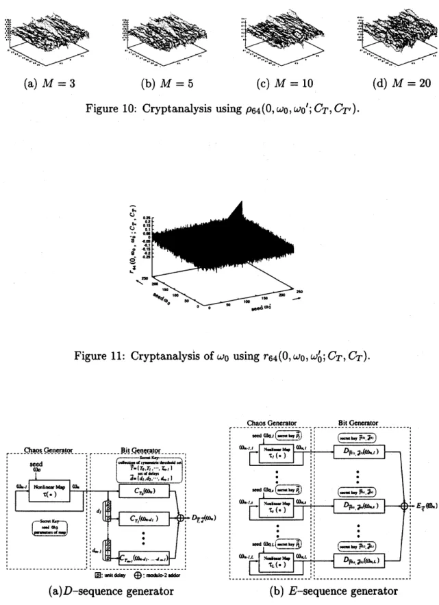
Figure 8: Cryptanalysis of$t_{M}$ using $\rho_{64}(0, \omega_{0}, \omega_{0;}C_{T}, C_{T},)$.

Figure 9: Cryptanalysis using$\rho_{64}(0,\omega_{0}, \omega 0’;\Theta_{t}, \Theta_{t},)$

.

an

initial seed $\omega_{0}$ and $\{G(\omega_{n}’)\}_{n=0}^{\infty}$ with anotherinitial seed

$\omega_{0’}$, defined by

$\rho_{N}(\ell, \omega_{0}, \omega_{0}’; F, G)=\frac{1}{N}\sum_{n=0}^{N-1}F(\omega_{n})G(\omega_{n+\ell}’)$ , (20)

where the subscripts

are

taken $\mathrm{m}\mathrm{o}\mathrm{d} N$

.

Note that $\mathrm{r}\mathrm{p}\mathrm{i}(1, \omega_{0}, \omega_{0}’;\ominus_{t}, _{t’})$has alargevalueonly

at$\ell=0$ because of its n0-correlation property. Figure 4showsautocorrelationfunctions with

theirn0-correlation property. Onthe other hand, thefluctuated and smooth

curves

inFigure

5indicate respectively the time-average $r_{64}(0, \omega_{0}, \omega_{0};_{t}, \ominus_{t’})$ of cross-correlation between

Qt(-) and $_{t’}(\cdot)$

versus

$t’$, and the ensemble-averaged

one

$\tilde{\rho}(0;\ominus_{t}$,easy. where $\tilde{\rho}(\ell;F, G)$ is

defined by

$\overline{\rho}(\ell;F, G)=\int_{J}F(\omega)G(\tau^{\ell}(\omega))f^{*}(\omega)$ du. (21)

Observethat thisfigureimpliesthat theestimationof the parameter$t$iseasyif the seed$\omega_{0}$ and

parameters ofthemap

are

previously knownandhencethat the key$t$ isnot cryptographically

secure

and should not be used. Thus the set ofthresholds, $T=\{t_{r}\}_{r=0}^{2M}$, may be used only

to satisfy the i.i.d. condition of sequences.

3.3

Cryptanalysis

3.3.1 Cryptanalysis of thresholds $t_{i}$

Figure 6and 7show searches ofthe thresholds $\{\mathrm{t}\mathrm{r}\}$ using cross-covariance functions

$\rho_{64}(0, \omega_{0}, \omega_{0}’;C_{T}, \ominus_{t})$, where $T=$

{0.3.0.6}

and $T=\{0.06,0.12,0.18,0.2,0.27,0.3,0.36,0.41$,

$\mathrm{e}.\mathrm{g}\cdot$,0.5, 0.6, 0.62, 0.65, 0.67,0.7,0.79, 0.89, 0.9,

0.96}

$(M=19)$, respectively and where $\omega_{0}’$ is

nearly equal to $\omega$ within (a) 7-bit precision, (b) 8-bit precision, (b) 9-bit precision, and (d)

10-bit precision. Observe that these figures imply that the

estimation

ofthe parameter $t$and

hence the estimation of the parameter $T=\{t_{r}\}_{r=0}^{2M}$ is easy if the seed $\omega_{0}$ and parameters

of the map

are

previously known. Unless $\omega_{0}’$ is equal to $\omega$, however, the search of $t$ is not

easy. Eventhough, the key $t$ is not cryptographically

secure

and should not be used. On the

contrary, the parameters $T$ may be used only to satisfy the conditions for asequence to be

one

of $i.i.d$

.

binary random variables. Figure 8shows $\rho_{64}(0, \omega_{0},\omega 0;C_{T}, C_{T’})$

versus

$t_{M}’$ to

search $t_{M}$, where $T=\{t_{r}\}_{r=1}^{M}$,$T’=\{t_{r}’\}_{r=1}^{M}$, and $\{t_{r}\pm\epsilon\}_{r=1}^{M-1}=\{t_{r}’\}_{r=1}^{M-1}$

.

3.3.2 Cryptanalysis of seed $\omega 0$

On the other hand, aseed $\omega_{0}$ ($i.e.$, an initial condition) is the best choice of asecret key in

stream cipher cryptography because of the SDIC(sensitive dependence

on

initialconditions)

property and the ergodicity of chaotic maps

as

discussed in Section 2. Figures 9shows

an

illustration of cryptanalysis using the statistics $r_{64}(0, \omega_{0}, \omega_{0}’;\theta_{t}, \theta_{t’})$, $r_{64}(0, \omega 0, \omega_{0}’;C\tau, C_{T’})$,

and $\rho_{64}(0, \omega_{0}, \omega_{0’};C_{T}, C_{T})$, respectively to search a10-digit seed $\omega_{0}=(0.0110100101)_{2}\simeq$

0.4113281.

.

., apartial secret key of abit sequence $\{C_{T}(\omega_{n})\}_{n=0}^{\infty}$ provided that all ofother

parameters

are

known within the limited accuracy, ($\omega_{0}’$ is nearly equal to $\omega$ within (a)

7-bit precision, (b) 8-bit precision, (c) 9-bit precision, and (d) 10-bit precision). In this

search all possible $2^{10}\omega_{0}’$’s

are

scanned. Figure 10 shows cryptanalysis of $t_{M}$ and $\omega 0$

us-ing $\rho_{64}(0, \omega_{0}, \omega_{0’};C_{T}, C_{T’})$, where $T=\{t_{r}\}_{r=1}^{M}$, $T’=\{t_{r}’\}_{r=1}^{M-1}$, and $\{t_{r}\}_{r=1}^{M-2}=\{t_{r}’\}_{r=1}^{M-2}$

.

Figure 11 shows cryptanalysis of$\omega_{0}$ using $r_{64}(0, \omega_{0}, \omega_{0}’;C_{T}, C_{T})$

.

We

can

find that

we

need

exhaustive searches of$\omega_{0}’$

even

if the parameters ofthe map, $e.g.$, degree$p$ of$T_{p}(\omega)$ and the

set

of

thresholds

are

previously known because $r_{64}(0, \omega_{0}, \omega_{0}’;C_{T}, C_{T})$ has apeak only when

$\mathrm{w}\mathrm{j}\ovalbox{\tt\small REJECT}\ovalbox{\tt\small REJECT}$ is equal to

$(\ovalbox{\tt\small REJECT}_{t})0$ completely in agiven precision [26]. This implies that this strategy is

computationally

infeasible

because of the large key

space

of$(\ovalbox{\tt\small REJECT}_{t})0$

.

3.4 Hierchical Structure

Achaotic

bit

sequence

$\{C_{T}(\omega_{n})\}_{n=0}^{\infty}$ is

asequence

of $i.i.d$

.

binary random variables under

certain conditions[23]. The $i.i.d$

.

property make it easier _{to construct chaotic bit}

genera-tors with hierarchical structures which

can

also produce sequences of $i.i.d$

.

binary random

variables. The first one, called level 1hierarchy, is based

on

the n0-correlation between

any

twosequences, $\{C_{T}(\omega_{n})\}_{n=0}^{\infty}$ and $\{C_{T’}(\omega_{n+\ell})\}_{n=0}^{\infty}$,

ffom

a

seed for $\ell\geq 1$

.

The n0-correlation

property between $\{C_{T}(\omega_{n})\}_{n=0}^{\infty}$ and $\{C_{T’}(\omega_{n}’)\}_{n=0}^{\infty}$ is defined by[23]

$\rho_{N}(\ell,\omega 0, \omega 0’;C_{T}, C_{T’})-\frac{1}{4}arrow(Q_{7\mathrm{T}’}-\frac{1}{4})\delta(\ell)\delta(\omega_{0}-\omega_{0}’)$ ,

as

$Narrow \mathrm{o}\mathrm{o}$ (22)

where$Q_{TT’}$ denotes anontrivial value which is afunction of$T$and$T’$

.

The second one, called

level 2hierarchy, is based

on

the n0-correlation between

any

two sequences ffom different

seeds. Such asequence $\{C_{T}(\omega_{n})\}_{n=0}^{\infty}$ is referred to

as

level 0hierarchy.

In order to increasethe number ofdifferent secret keys,

we can use

the modulo2addition

ofchaotic symmetricbinary sequences $\{C_{T_{j}}(\omega_{n})\}_{n=0}^{\infty}$ with asymmetric threshold set

$T_{j}=\{t:(j)\}_{\dot{|}=0}^{2M(j)}$, _{$0\leq j\leq m-1$}

.

(23)

For apositive integer

₄

$(1 \leq i\leq m-1)$,

we

get

$D_{\vec{T},\overline{d}}\{\omega_{n}$) $=\mathrm{C}\mathrm{T}\mathrm{o}\{\mathrm{u}\mathrm{n}$) $\oplus C_{T_{1}}(\omega_{n-d_{1}})\oplus\cdots\oplus C_{T_{m-1}}(\omega_{n-d_{1}-\cdots-d_{m-1}})$, (24)

$\vec{T}=\{T_{0},T_{1}, \cdots,T_{m-1}\}$, $\vec{d}=\{d_{1},d_{2}, \cdots, d_{m-1}\}$ (23)

which is obtained from achaotic real-valued trajectory $\{\omega_{n}\}_{n=0}^{\infty}$

as

shown in Figure 12 (a).

Note that

{

$D_{\vec{T},\vec{d}}\{\omega)\}_{n=0}^{\infty}$ is also

asequence

of $i.i.d$

.

binary random variables.

Hence

we

call

such asequence

_{

$D_{f,\overline{d}}\{\omega)\}_{n=0}^{\infty}$

a

generalized version

of

chaotic symmetric binary sequences.

For such asequence,

we

can use

not only $\vec{T}$

but also $\vec{d}\mathrm{a}\mathrm{s}$

secret keys.

For$L$seedswhich

are

chosen statistically independently andfor$L$ergodicmaps,

we

define

$E_{\vec{\tau}}(\vec{\omega_{n}})=D_{\vec{T}(1),d11)(\omega_{n,1})\oplus D_{\vec{T}(2),d\mathrm{t}2)(\omega_{n,2})\oplus\cdots\oplus D_{\vec{T}(L),d1\iota)}(\omega_{n,L})}}$ (26) $\vec{\tau}=\{\tau_{1}, \tau_{2}, \cdots, \tau_{L}\}$, $\vec{\omega_{n}}=\{\omega_{n,1}, \omega_{n,2}, \cdots,\omega_{n,L}\}$, $\omega_{n,s}=\tau_{s}^{n}(\omega_{0,s})$ (27)

The additive property of$i.:.d$

.

binary random variables aUows

us

_{to get} asequence of$i.i.d$

.

binary random variables $\{E_{\vec{\tau}}(\vec{\omega}_{n})\}_{n=0}^{\infty}$

as

shown in Figure 12. Note that periods of such

sequences canbe longerthanonesof each real-valuedsequences $\{\omega_{n,s}\}_{n=0}^{\infty}$in afinite precision

computation system. Figure 12 shows (a) abit generator $D_{\vec{T},d}\prec\omega$) and (b) abit generator

$E_{\vec{\tau}}(\vec{\omega}_{n})$, respectively.

4Concluding Remarks

Nevertheless, it is hardto prove that suchasystem implemented in afloating-point

environ-ment is cryptographically

secure

from the cryptographic point of view: $e.g.$, the period of

a

running sequence generatedby this cryptosystemis short.

Some

cryptographic problems

can

be settled only if

progress

in

some

number-theoretic problems $\mathrm{a}\mathrm{n}\mathrm{d}/\mathrm{o}\mathrm{r}$ information theoretic

ones can

be made. Lastly note that most of the existing chaos cryptosystems have been

incapable of fully utilizing the sensitive dependence on initial conditions property, Le., $\omega_{0}$,

primarily because they

are

based

on

analog circuits

(a) M $=3$ (b) _$M=5$ (c) M $=10$ (d) M $=20$

Figure

10:

Cryptanalysis using $\rho_{64}(0,\omega_{0},\omega_{0’};C_{T}, C_{T’})$

.

Figure 11: Cryptanalysis of$\omega_{0}$ using $r_{64}(0, \omega_{0}, \omega_{0}’;C_{T}, C_{T})$

.

$(\mathrm{a})D$-sequence generator (b) $E$

-sequence

generator

Figure 12: Hierachicalsequence generator

References

[1] M. Kac,

_{“Statistical}

_{Independence in}

_Probability

_{Analysis and}

_Number

_Theory,”

_The

Mathematical Association

ofAmerica,

1959.

[2] M. Loeve, “ProbabilityTheory I,”

Graduate

Texts in

Mathematics

45,

Springer-Verlag,

1977.

[3] P. _{Billingsley, “Probability and Measure,” John Wiley&Sons,}

_1995.

[4] P.R. Halmos, “Lectures

on

Ergodic Theory,” The

Mathematical

SocietyJapan,

1956.

[5] A. J. Viterbi and J. K. Omura, “Principles of Digital

Communication

and Coding,”

McGraw-HillBook Company, Tokyo,

1979.

[6] _{J. L. Massey, “An introduction to contemporary cryptology,” Proc. IEEE, 76, n0.5,}

533-549, May

1988.

[7] T.W. Cusick, C.Ding, and A.Renvall, “Stream _{Ciphers and Number Theory,” North}

Holland,

1998.

[8] J.

von

Neumann, Summary written by G. E. Forsythe, “Various techniques used in

connection with random digit”, National Bureau

_of

Standards, Applied Math. Series,

12, 36-38,

_1951.

[9] D. Knuth, “The Art of Computer Programming 2,

Seminumerical

Algorithms,” 2nd ed.,

Addison-Wesley, Reading, Mass, 1981.

[10] D. V. Sarwate and M. B. Pursley,

“Crosscorrelation

properties of pseudorandom and

relatedsequences,” Proc. IEEE, 68, n0.3, 593-619,

1980.

[11] S. M. Ulam and J.von Neumann, “On combination ofstochastic and deterministic

pr0-cesses”, Bull. Math. Soc. 53, pp.1120,1977.

[12] R.A. Matthews, “On the derivation of a“chaotic” encryption _{algorithm,” Cryptologia,}

13,pp.29-42,

1989.

[13] D.D. Wheeler and R.A. Matthews, _{“Supercomputer Investigations of achaotic}

encryp-tion algorithm,” Cryptologia, 15,pp.140-152, April, 1991.

[14] T.Habutsu, Y.Nishio, I.Sasase and _{S.Mori, “A secrete key cryptosystem by}

iter-ating achaotic map,” in Proc. Advances in $C\eta ptology$

-EUROCRYPT’91.

Berelin,

Germany:Springer-Verlag,1991,

pp.

127-140.

[15] M. Gotz, K. Kelber, andW. Schwarz,

“Discrete-time

chaotic encryption systems part I:

statistical design approach” IEEE Trans.

Circuit

Syst, CAS-44, n0.5,

963-970, 1997.

[16] F. Dachselt, K. Kelber, and W. Schwarz, _{“Discrete-time chaoticencryption systems part}

III: cryptographical analysis” IEEE Rans.

Circuit

Syst, CAS-45, n0.9, pp.983-988,

1998.

[17]

M.S.

Bapista, “Cryptography with chaos,” Phys. Lett.A, 240, pp.5-54.

1998.

[18] G. Jakimoski and L. Kocarev, “Chaos _{and cryptographyrblock encryption ciphers based}

on

chaotic maps,” IEEE $\mathfrak{R}ans$

.

Circuit

Syst, CAS-48, n0.2, pp.163-169,

2001

[19] T. Kohda, A. Tsuneda, and T. Sakae, “Chaotic Binary Sequences by Chebychev Maps

and Their Correlation Properties”,Proc.

_of

the IEEE Second Int. Sympo. on Spread

Spectrum Techniques and Applications, 63-66,

1992.

[20] T. Kohda and A. Tsuneda, “Pseudonoise

sequences

by chaotic nonlinear maps andtheir

correlation properties,”

IEICE

Trans. Communications, E76-B, n0.8, 855-862,

1993.

[21] T. Kohda and A. Tsuneda, “Explicit evaluations of correlation functions of Chebyshev

binary and bit

sequences

based

on Perron-Frobenius

operator,” IEICE., Trans.

Funda-mentals, E77-A,

no.

11, 1794-1800,1994.

[22] D.S. Broomhead, J.P. Huke, and M.R. Muldoon, “Codes for spread spectrum

applica-tions generatedusing chaotic dynamical systems. Dynamics and Stability

of

Systems,14,

pp.95-105,1999.

[23] T. Kohda and A. Tsuneda, “Statistics ofchaotic binary sequences”, IEEE Trans.

Infor-mation Theory, 43, no.1, 104-112, 1997.

[24] T. Kohda, “Sequences of i.i.d. binary random variables using chaotic dynamics”,

Se-quences and Their Applications, eds. by C. Ding, T. Helleseth, and H. Niederreiter,

297-307, Springer-Verlag, 1999.

[25] T.Kohda and A.Tsuneda, “Chaotic Bit Sequences for Stream Cipher Cryptographyand

Their Correlation Functions” , Proc. SPIE’s Photonics East ’95 Sympo. (Chaotic Circuit

for Communication), SPIE Vo1.2612, PP.86-97, 1995.

[26] T. Kohda and A. Tsuneda, “Stream cipher systems based on chaotic binary

se-quences”,Proc. the 19996 Symp. on Cryptography and

Information

Security,

SCIS96-11 , pp.1-8, 1996.

[27] O. W. Rechard, “Invariant

measures

for many-0ne transformation,” Duke Math. J., 23

pp.477-488, 1956.

[28] A. Lasota and M. C. Mackey, Chaos, Fractals, and Noise, Springer-Verlag,

1994.

[29] R. L. AdlerandT. J.Rivlin, “Ergodic and mixingproperties ofChebyshevpolynomials,”

Proc. Amer. Math. Soc, 15, 794,

1964.

[30] T. J. Rivlin, “Chebyshev polynomials,”, John Wiley&Sons, Inc., 1990.

[31] S. Grossmann and S. Thomae, “Invariant distributions and stationary correlation

func-tions ofone-dimensional discrete processes,” Z. Naturforsch., 32a, 1353-1363, 1977.

[32]

B.O.

Koopman, “Hamiltonian systems and

transformations

in Hilbert space” ,

Proc. Natl.Acad.Sci., U.S.A.,17,pp.315-318,1931