Construction of diffusion processes penetrating fractals : An application of the theory of Besov spaces (Harmonic Analysis and Nonlinear Partial Differential Equations)

Construction of

diffusion

processes

penetrating

fractals

-

An

application

of the theory of

Besov spaces

-Takashi

Kumagai

*

熊谷

隆

(

京都大学数理解析研究所

)

1

Introduction

Assume thatthere are countable number of disordered media $\{K\dot{.}\}_{=1}^{M}\dot{.}(1\leq M\leq$

$\infty)$ on $\mathrm{R}^{N}$

.

Can we construct adiffusionprocess which

moves

the whole space,

whose behaviour islikeBrownian motionon$K_{i}$ foreachmedia and like Brownian

motion on$\mathrm{R}^{N}$

outside? If

we

can, howdoesthediffusionbehave asymptotically? In this paper,

we

will treat this problem when $K_{i}$’s

are

fractals.

Since late $80’ \mathrm{s}$, there have been many works for diffusion processes and

Laplace operators

on

fractals (see [1], [9], [11] e.t.c). Recent works ([6], [7], [10]$)$ reveal that domains of the corresponding quadratic forms (Dirichlet forms)

are Besov spaces andthat theories of Besov spacescould be applied to this field. Our work shows that $\mathrm{t}\mathrm{r}\mathrm{a}\mathrm{c}\mathrm{e}$ theory of Besov spaces is applicable to the question

posed.

The initialwork

on

diffusionprocesses penetratingfractals

was

by$\mathrm{L}\mathrm{i}\mathrm{n}\mathrm{d}\mathrm{s}\mathrm{t}\mathrm{r}\emptyset \mathrm{m}$ [14] and has been followed up by

more

general constructions in [7], [10]. These

’Research Institute for Mathematical Sciences, Kyoto University,

Kyoto 606-8502, Japan. $\mathrm{E}$-mail:[email protected] 数理解析研究所講究録 1235 巻 2001 年 91-114

papers have been primarily interestedindemonstrating theexistence ofaprocess

whichbehaves like adiffusion

on

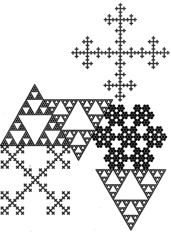
afractalwithin asubset ofEuclideanspace, yet

standard Brownian motion outside. Our work will extend this construction to

incorporate many different fractals which may be embedded in

some

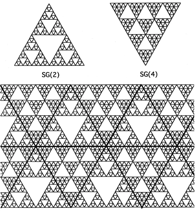
Euclidean

space (Figure 2), but also may tile the space (Figure 1). We will call spaces of

either type

_{fractal fields.}

Akey examplethat

we

would like the reader to bear inmind throughout the paper is the gasket tiling in $\mathrm{R}^{2}$

.

Consider atriangular

lattice

on

$\mathrm{R}^{2}$ where each

edge is of length 1. We will fill each triangle with aversion of the Sierpinski

gasket in periodicway. Moreprecisely, let $SG(l)$ be thefamilyof2-dimensi0nal

Sierpinski gaskets from [3] with sidelength 1constructed by contraction maps

with contraction factor 1/1. Now, takeaset of triangles (welet $L$ be thenumber of triangles in the set) from the triangular lattice

so

that the union of them is

aconnected closed set. In each triangle

we

place $\{SG(l_{k})\}_{k=1}^{L}$ and denote the

union of these fractals by $K_{0}$

.

Without loss of generality,

we can

assume

that

one

oftheverticesof$K_{0}$ is $(0, 0)$

.

We take $i_{x}\in \mathrm{N}$

so

that $\mathrm{K}\mathrm{o}(K_{0}+(\mathrm{i}\mathrm{x}, 0))\neq\emptyset$ and Int $K_{0}\cap \mathrm{I}\mathrm{n}\mathrm{t}$ $(K_{0}+(i_{x},0))=\emptyset$

.

We also take _{$i_{y}\in \mathrm{N}$} in the

same

way by

taking $(0, i_{y})$ instead of$\langle$$i_{x},0)$

.

Then, _{$G \equiv\bigcup_{l,m\in}\mathrm{z}(K_{0}+(li_{x},mi_{y}))$} is the space

we

will consider. Figure 1indicates the

case

when $K_{0}$ is aparalelogram filled

with $SG(2)$ and $SG(4)$

.

This paper will treat the general construction problem. We incorporate the

$\mathrm{t}\mathrm{r}\mathrm{a}\mathrm{c}\mathrm{e}$ theory of Besov spaces, for the embedding

into aEuclidean space, with

an

idea originally due to Kusuoka, [12] which shows how to extend aLipschitz

function from the boundary of afractal to the interior while controlling its

energy. This will allow

us

to build up aDirichlet form and establish

some

properties, such

as

aNash inequality. In the forthcoming paper [5], we will

further discuss

on

_{heat kernel estimates and the large}

_deviations

_of

_our

_diffusion

process. In the paper, we will

demonstrate

the shape of the shortest paths

through

our

_{fractal fields and observe thatit isfractals with small} $d_{w}$ which take

the longest to

cross

(in_{the short time}limit) andthis allows

us

to

determine

the

shortest paths _{in arecursive manner, first fixing them through the slow parts}

and filling inthe details for the faster paths.

2Fractal fields

and

_{their Dirichlet forms}

In this section we will introduce fractal fields, the framework within which we

will work. Our aim is to construct local regular _{Dirichlet forms on these spaces.} Let $\{K_{i}\}_{i=1}^{M}\subset \mathrm{R}^{2}(1\leq M\leq\infty)$ be afamily of(bounded or

unbounded) nested

fractals whose definition will be given in Appendix. When $K_{i}$ isunbounded, we

denote by $\hat{K}_{i}$ the

corresponding bounded nested fractal (when $K_{i}$ is bounded,

$\hat{K}_{i}=K_{i})$ and denote by $\{\Psi_{j}^{(i)}\}j\in s\dot{.}$ the family of contractions

which determine

$\hat{K}_{i}(S_{i}=\{1,2, \cdots,N_{i}\})$

.

Let $V_{0}^{(i)}$ be the

set of essential fixed points for $\hat{K}_{i}$.

For each closed set $A$, let Cov (A) be the set of _points

covered by $A$, i.e., decomposing $\mathrm{R}^{2}\backslash A$ into connected components

$\{D_{j}\}_{j=1}^{\infty}$ and denoting by

$\{Dj\}j\in U(A)$ the unbounded components, Cov $(A)= \mathrm{R}^{2}\backslash \bigcup_{j\in U(A)}D_{j}$

.

We note

that ifthe set $A$ has holes, these may be contained

in Cov(A). We

assume

the

followingfor the location of $\{K_{i}\}_{i}$

.

Assumption 2.1 1) For each $1\leq i\neq j\leq M$,

Int (Cov $(K_{i}))\cap Int$ (Cov $(K_{j}))=\emptyset$,

where Int (K) is the interior

_of

K.

2) For each compact set $C\subset \mathrm{R}^{2}$,

$\#\{i:C\cap K_{i}\neq\emptyset\}<\infty$

.

Define $G= \bigcup_{i=1}^{M}K_{i}$ and $D=\mathrm{R}^{2}\backslash \mathrm{C}\mathrm{o}\mathrm{v}(G)$ , then $G$ is aclosed set by 2) of

Assumption 2.1. Clearly, $D= \bigcup_{j\in U(G)}D_{j}$

.

We define $\tilde{G}=G\cup D$ and call it a

fractal field

generated by $\{K_{\dot{2}}\}_{i=1}^{M}$

.

See Figure 1and Figure 2for examples of fractal fields. Note that we

can

define fractal fields

on

$\mathrm{R}^{N}$ in the

same

way using

nested fractals

on

$\mathrm{R}^{N}$, but

as our

Assumption2.2, which will be introducedlater,

seldom holds for nested fractals

on

$N\geq 3$,

we

will restrict to $N=2$

.

Let $\partial_{e}G$ be the topological boundary of $G$

as

asubset of R. For $1\leq i\neq$

$j\leq M$, let

$\Gamma_{ij}=\mathrm{C}\mathrm{o}\mathrm{v}$ $(K\dot{.})\cap \mathrm{C}\mathrm{o}\mathrm{v}$ $(K_{j})$, $\partial_{i}G=\bigcup_{1\leq:\neq j\leq M}\Gamma_{ij}$

.

(2.1)

Set $\partial G=\partial_{e}G\cup\partial\dot{.}G$

.

Let $\mu$

:be

normalized Hausdorff

measure on

$K_{i}$, i.e.

$\mu:(\hat{K}\dot{.})=1$, and set $\mu=\Sigma_{i=1}^{M}\mu\dot{.},\tilde{\mu}=m|_{D}+\mu$ where

m

isthe Lebesgue measure

on

R.

We next define aform

on

$\tilde{G}$

.

First, for each $i$, the local regular Dirichlet

form $(\mathcal{E}_{K}F_{K}.):’$

.on

$\mathrm{L}^{2}(K_{i,\mu:})$ is given

as

in Theorem A.2 and Theorem A.5.

We denote $d_{f}(K_{i}),d_{s}(K.\cdot),d_{w}(K_{i})$ the Hausdorff, spectral and walk dimension

respectively w.r.t. Euclidean metric. Let $K\subset K_{i}$ be acompact nested fractal

which is congruent to $\hat{K}\dot{.}$ (thus, when

$K\dot{.}$ is bounded, $K=K_{i}$). For each $\Gamma_{ij}$ in

(2.1) where $1\leq i\neq j\leq M$ and for $\omega$ $\in\Sigma_{:}\equiv(S_{i})^{\mathrm{N}}$, let $d_{\Gamma_{\mathrm{j}},K}. \cdot(\omega)=\min\{n\geq$

$1$ : $\Gamma_{\dot{|}j}\cap\Psi_{\omega_{1}\cdots\omega_{n}}^{(K)}(K)=\emptyset\}$ where $\{\Psi_{j}^{(K)}\}_{j\in S}.\cdot$ is afamily of $\mathrm{a}\mathrm{i}$-contractions which

determine $K$, and define

$\kappa(\Gamma_{\dot{|}j}, K)=-\lim\sup\log\nu\dot{.}(d_{\Gamma_{j\prime}K}.\cdot(\omega)>n)\underline{1}\underline{1}$,

$\log N_{i}narrow\infty n$

where $\nu_{i}$ is aBernoulli

measure

on $\Sigma_{i}$

so

that _{$\nu_{i}(\{\omega\in\Sigma_{i} : \omega_{1}=l\})--1/N_{i}$} for

each $\mathit{1}\in S_{i}$. We adopt the convention that -logO _$=\infty$.

Assumption 2.2 For each $1\leq i\neq j\leq M$, the following holds where K and

$Yij$ are

as

above,

$\frac{2}{d_{s}(K)}-\frac{2}{d_{f}(K)}<\kappa(\Gamma_{ij}, K)$. (2.2)

Remark 2.3 For the gasket tiling introduced in the Introduction (also indicated in Figure $\mathrm{I}$), (2.2) always holds.

Indeed, let $K=SG(l)l\geq 2$ and $\Gamma=\Gamma_{ij}$ be the bottom line

_of

K. As there are$l^{n}n$-cells which intersect with $\Gamma$, we see that

$\nu(d_{\Gamma,K}(\omega)>n)=l^{n}/L^{n}$ where $L–l(l+1)/2$ . Thus, $\kappa(\Gamma, K)--1-\log l/\log L$

and (2.2) is equivalent to

$\frac{\log(\rho L)-2\log l}{1\mathrm{o}\mathrm{g}L}<1-\frac{1\mathrm{o}\mathrm{g}l}{1\mathrm{o}\mathrm{g}L}$,

which is equivalent to $\rho<l$

.

Note that $\rho=P^{x_{0}}(\tau_{V_{0}}\backslash \{x_{0}\}(X)<\tau_{x\mathrm{o}}(X))^{-1}$ where

$x_{0}\in V_{0},$ $X$ is a Markov chain $co$ responding to $(\mathcal{E}_{SG(l)})_{1;}$ and $\tau_{A}(X)$ is the

first

hitting time

_of

$X$ to A. Note also that

if

we

define

$\overline{X}$

be a simple random walk on $\mathrm{Z}$, then _{$l=P^{0}( \tau\{-\iota,\iota\}(\overline{X})<\inf\{n\geq 1 : \overline{X}(n)=0\})^{-1}$}. Then, by the

comparison

of

escape probabilities using the electrical network method (we use

so called cutting law), we can easily obtain $\rho<l$

.

Assumption 2.1 and Assumption 2.2 will hold throughout the paper. We define abilinear form $(\tilde{\mathcal{E}}, D(\tilde{\mathcal{E}}))$ on $\mathrm{L}^{2}(\tilde{G},\tilde{\mu})$ as follows,

$\tilde{\mathcal{E}}(u, v)$ _{$= \sum_{i=1}^{M}\mathcal{E}_{K}(:u|_{K_{i}},v|_{K:})+\frac{1}{2}\sum_{j\in U(G)}\int_{D_{j}}\nabla u(x)\nabla v(x)dx$} for all

$u$,$v\in D(\tilde{\mathcal{E}})$,

$D(\tilde{\mathcal{E}})$ _{$=$ $\{u\in C_{0}(\tilde{G}) : u|_{K}:\in F_{K}.\cdot\forall i, u|_{D_{j}}\in W^{1,2}(D_{j})\forall j,\tilde{\mathcal{E}}(u,u)<\infty\}$},

where $D= \bigcup_{j\in U(G)}D_{j}$is adecomposition of $D$ into open connectedcomponent$\mathrm{s}$

and $C_{0}(\tilde{G})$ is aspaceofcontinuous functions on$\tilde{G}$

withcompact support. Then,

it is easy to check the following.

Lemma 2.4 1) $(\tilde{\mathcal{E}}, D(\tilde{\mathcal{E}}))$ is closable in $\mathrm{L}^{2}(\tilde{G},\tilde{\mu})$

.

2) $D(\tilde{\mathcal{E}})$ is

an

algebra.

3) For each$j$, _{$x\in K_{j}$} and each $U(x)$ which is

a

neighborhood

of

$x$, there xists $f\in F\kappa_{\mathrm{j}}\cap C_{0}(K_{j})$ such that $f(x)>0$ and Supp _{$f\subset U(x)\cap K_{j}$} where Supp _$f$ denotes the support

_of

$f$

.

4) $C_{0}^{\infty}(D)\subset D(\tilde{\mathcal{E}})$

.

Now, denote$\tilde{F}=\overline{D(\tilde{\mathcal{E}})}^{\overline{\mathcal{E}}_{(1)}}$

so

that $(\tilde{\mathcal{E}},\tilde{F})$ is the smallest extension of $(\tilde{\mathcal{E}},D(\tilde{\mathcal{E}}))$,

where $\tilde{\mathcal{E}}_{(1)}(f, f)=\tilde{\mathcal{E}}(f, f)+||f||_{\mathrm{L}^{2}(\overline{G},\overline{\mu})}^{2}$

.

We then have the following. Theorem 2.5 $(\tilde{\mathcal{E}},\tilde{F})$ is

a

$local$ regularDirichlet

form

on

$\mathrm{L}^{2}(\tilde{G},\tilde{\mu})$

.

Bythegeneral theory ([2]), there is

aone

to

one

correspondence between alocal

regular Dirichlet form

on

$\mathrm{L}^{2}(\tilde{G},\tilde{\mu})$ and

a

$\mu\sim$-symmetric diffusion process on $\tilde{G}$

except for

some

exceptional set of starting points. We will denote by $\{\tilde{X}_{t}\}_{t\geq 0}$

the diffusion process corresponding to $(\tilde{\mathcal{E}},\tilde{F})$

.

Note that,

as

the original

forms on $\{K\dot{.}\}$

:and

$\{D_{j}\}_{j}$

are

strong local, $(\tilde{\mathcal{E}},\tilde{F})$ is also strong local.

For the proof ofTheorem 2.5, the keypart is to prove the following.

Proposition 2.6 1) For each $x\neq y\in\tilde{G}$, there $n\cdot s\$ $g\in D(\tilde{\mathcal{E}})$ such that $g(x)\neq g(y)$

.

2) For

any

compact set $L$ in $\tilde{G}$, there exists

$f\in D(\tilde{\mathcal{E}})$ such that _{$f|_{L}=1$}

.

Indeed, usingthisproposition,

we can

prove Thorem 2.5

as

follows. It is easy to

see

that $(\tilde{\mathcal{E}},\tilde{F})$ is alocal Dirichlet form. Also,

as

$\tilde{F}=\frac{-}{D(\tilde{\mathcal{E}})}(1)$

, it is clear that

$D(\tilde{\mathcal{E}})$ is dense in $\tilde{F}$

w.r.t. $\tilde{\mathcal{E}}_{(1)}$

-norm.

Thus, all

we

need for the regularity

ofthe

form is to show that $D(\tilde{\mathcal{E}})$ is dense in _{$C_{0}(K)$} w.r.t.

$||\cdot||_{\infty}$

-norm.

Now,

as

$D(\tilde{\mathcal{E}})$

is an algebra (Lemma 2.42)$)$,

we see

that for each compact set $L$ in $\tilde{G}$

, $D(\tilde{\mathcal{E}})|_{L}$

is dense in $C(L)$ by using Proposition 2.6 and applying the Stone-Weierstrass

theorem. This establishes regularity and we have completed the proof.

For each $B\subset \mathrm{R}^{2}$, define _{$\tau_{B}=\inf\{t\geq 0:\tilde{X}_{t}\in B\}$}

.

We

can

then prove that

$\tilde{X}_{t}$ penetrates into each

$K_{i}$

.

To say

more

exactly, we have the following.

Proposition 2.7 Assume that $m(G)=0$ where $m$ is the Lebesgue

measure on

R. Then,

_for

any nearly Borel set B with positive $l$-capacity $(w.r.t.\tilde{\mathcal{E}})$,

$\tilde{P}^{x}(\tau_{B}<\infty)>0$

for

quasi-every x$\in \mathrm{R}$

.

(2.3)

Especially, when$B$ is either

a

subset

of

$K_{i}$ whose$l$-capacity $w.r.t$. $\mathcal{E}_{K}\dot{.}$ ispositive

or a subset

_of

$\mathrm{R}^{2}$ whose _$l$-capacity

$w.r.t$

.

the Dirichlet integral is positive, then

(2.3) holds.

The proofis the same as Proposition 2.9 in [10].

In the

same

way as Theorem 2.11 in [10], we

can

prove aNashtype estimate

for the heat semigroup. Let $P_{t}^{\overline{\mathcal{E}}}(t>0)$ be the semigroup corresponding to

$(\tilde{\mathcal{E}},\tilde{F})$

.

Then, the following holds (see [10] for the proof).

Proposition 2.8 Assume

_further

that there

are

only

_finite

types in $\{K_{i}\}_{i=1}^{M},$ $i.e$.

if

we

_define

that two $K_{i}’ s$ which are similar

are

equivalent, there

are

only

finite

number

_of

equivalence classes in $\{K_{i}\}_{i=1}^{M}$

.

Define

$d_{s}^{\min}= \min_{i=1}^{M}d_{s}(K_{i})$

.

Then,

there exists $c_{2.1}>0$ such that thefollowing holds

for

all $x,y\in\tilde{G}$,

$||P_{t}^{\overline{\mathcal{E}}}||_{1arrow\infty}\leq\{$

$c_{2.1}t^{-1}$,

for

all _$t\in(0,1]$,

$c_{2.1}t^{-d_{\epsilon}^{\min}/2}$,

for

all $t\in[1, \infty)$

.

(2.4)

3Proof of Proposition 2.6

In this section,

we

will give aproof of Proposition 2.6. The crucial part is to

show 1) for the

case

$x\vee y\in\partial\dot{.}G$ and $x\vee y\in\partial_{e}G$, where $x\vee y$

means

$x$

or

$y$

.

We adopt completely different methods for the two cases;

we

use

self-similarity

and nesting property for the former

case

and for the latter case,

we

apply the

extension operator used in the $\mathrm{t}\mathrm{r}\mathrm{a}\mathrm{c}\mathrm{e}$ theory of Besov spaces.

We will first prove 1) for the

case

$x\vee y\in\partial_{\dot{1}}G$

.

Assumption 2.2 will be used

here. For each $f\in C(\mathrm{R}^{2})$, let $||f|| \mathrm{L}\mathrm{i}\mathrm{p}=\sup\{|f(x)-f(y)|/||x-y|| : x,y\in \mathrm{R}^{2}\}$

and let Lip $(\mathrm{R}^{2})=\{f\in C(\mathrm{R}^{2}) : ||f||\mathrm{L}\mathrm{i}\mathrm{p}<\infty\}$

.

We

now

give

an

important

lemma due essentialy to Kusuoka ([12]).

Lemma 3.1 For each $\Gamma_{\dot{|}j}$ in (2.1) where $l\leq i\neq j\leq M$ and

for

each $K\subset K_{i}$ which is congruent to $\hat{K}.\cdot$ and _{$K\cap\Gamma_{j}.\cdot\neq\emptyset$}, let

$H_{\Gamma_{j},K}.\cdot$ : Lip $(\mathrm{R}^{2})arrow C(K)$ be $a$

linear operator given by

$H_{\Gamma_{j},K}\dot{.}g(x)=E^{x}[g(X_{\tau_{\Gamma_{j}}}\dot{.})]$,

for

all $x\in K$, $g\in Lip$ $(\mathrm{R}^{2})$ (3.1)

where $\{X_{t}\}$ is the Brownian motion

on

$K$ and $\tau \mathrm{r}_{\mathrm{j}}.\cdot=\inf\{t\geq 0 : X_{t}\in\Gamma_{ij}\}$. Then, $H_{\Gamma_{j},K}.\cdot g\in F_{K}$

.

$h\hslash her$, there eists $c_{2.2}=c_{2.2}(K)>0$ such

tteat

$\mathcal{E}(H_{\Gamma_{\mathrm{j}\prime}K}.\cdot g, H_{\Gamma_{j\prime}K}.\cdot g)\leq c_{2.2}\{\int_{\Sigma}\dot{.}(\rho:L:\alpha_{i}^{-2})^{d_{\Gamma_{j\prime}K}(\cdot)}.\cdot\nu(\mathrm{d}v)\}||g||_{Lip}^{2}$ (3.2)

holds

_for

any $g\in Lip$ $(\mathrm{R}^{2})$

.

PROOF. In the following,

we

will abbreviate $\Gamma_{j}.\cdot$ to $\Gamma$ and

remove

the

sub-scripts i and K. For each g $\in C(K)$, define $h_{\Gamma}(\cdot$: g):K $arrow \mathrm{R}$ as follows,

$h_{\Gamma}(\pi(\omega) : g)=\{$

$E^{\pi(\sigma^{m}\omega)}[g\circ\Psi_{\omega_{1}\cdots w_{m}}(X_{\tau_{\mathrm{V}_{0}}})]$ if $d\mathrm{r}(\omega)=m$,

$g(\pi(\omega))$ if $d_{\Gamma}(\omega)=\infty$,

(3.3)

for each $\omega\in\Sigma$ (see the Appendix for the notation). It is easy to

see

that

$\mathrm{h}\mathrm{r}(- :g)$ is

awell-defined

continuous map which is harmonic inside $\Psi_{\omega_{1}\cdots\omega_{m}}(K)$

if$\mathrm{d}\mathrm{v}(\mathrm{u})=m$, and $h_{\Gamma}(\cdot :g)|_{\Gamma}=g|\mathrm{r}$

.

Moreover, noting that

$\mathcal{E}_{n}(g)=\rho^{n}\sum_{w\in S^{n}}$each

$\mathrm{o}\Psi_{w}$) for all $g\in C(V_{n})$,

where we abbreviate $\mathcal{E}_{n}(g,g)$ to $\mathcal{E}_{n}(g)$, we

can

easily

see

that

$\mathcal{E}_{n}(h_{\Gamma}(\cdot : g)|_{V_{n}})=\int_{\Sigma}\rho^{d_{\Gamma}((v)\wedge n}\cdot L^{d_{\Gamma}(v)\wedge n}‘ \mathcal{E}_{0}(\{g(\pi([\omega,i]_{d_{\Gamma}(\omega)\wedge n}));i\in S\})\nu(h)$ , (3.4)

where we set $[\omega, i]_{l}=\omega_{1}\cdots\omega_{l}ii\cdots$. Note also that there exists $c_{1}>0$ such that

$c_{1}^{-1} \mathcal{E}_{0}(u)\leq\max\{|u(x)-u(y)|^{2} : x,y\in V_{0}\}\leq c_{1}\mathcal{E}_{0}(u)$ (3.5)

for any $u\in C(V_{0})$

.

Using (3.4), (3.5) and the fact $\rho L\alpha^{-2}>1(,\mathrm{w}\mathrm{h}\mathrm{i}\mathrm{c}\mathrm{h}$ is shown

in [1], Proposition 6.30), we have foreach $g\in C(K)$ that

$\mathcal{E}_{n}(h_{\Gamma}(\cdot :g)|_{V_{n}})$ $\leq$ $c_{1} \cdot\{\int_{\Sigma}(\rho L\alpha^{-2})^{d_{\Gamma}((\psi)}\nu(d\omega)\}$

$\cross$ $\sup_{m}\{\alpha^{m}\cdot\max\{|g(x)-g(y)| : x, y\in V_{\xi}\};m\geq 0,\xi\in S^{m}\}^{2}$

.

On the otherhand,from Assumption 2.2, we see that $A= \int_{\Sigma}(\rho L\alpha^{-2})^{d_{\Gamma}(\omega)}\nu(h)<$

$\infty$. We thus obtain

$\mathcal{E}(h_{\Gamma}(\cdot :g), h_{\Gamma}(\cdot : g))\leq c_{1}\cdot A$

.

$\{$

diain

$K\}^{2}\cdot||g||_{\mathrm{L}\mathrm{i}\mathrm{p}}^{2}$,

for each $g\in \mathrm{L}\mathrm{i}\mathrm{p}(\mathrm{R}^{2})$

.

As

$\mathcal{E}(H_{\Gamma,K}g, H_{\Gamma,K}g)=\inf\{\mathcal{E}(u,u) : u\in F, u|_{\Gamma}=g\}$ for all $g\in \mathrm{L}\mathrm{i}\mathrm{p}(\mathrm{R}^{2})$,

we obtain the desired facts.

:

Using this, we now show 1) of Proposition2.6 for the

case

$x\vee y\in\partial_{i}G\backslash \partial_{e}G$.

Proposition 3.2 For each $x\neq y\in\tilde{G}$ there $x\in\partial_{i}G\backslash \partial_{e}G$, there exists _$f\in$

$D(\tilde{\mathcal{E}})$ such that $f(x)=1$,$f(y)=0$

.

Proof. For $x\in\partial\dot{.}G\backslash \partial_{\mathrm{e}}G$, denote $\{K_{i}\}_{i\in I(x)}$ the set of all $K_{i}$ such that

$x\in K_{i}$

.

For each $K\dot{.}i\in I(x)$, take $m:\in \mathrm{N}$ such that $\alpha_{i}^{-m_{t}-1}\leq e^{-m}<\alpha_{j}^{-m}$:and define $N_{m}(x)$

as

aunion ofthe $m_{i}$-complexes which contain $x$ for each $i\in I(x)$

.

Also, define $N_{m}^{1}(x)$

as

aunion of the $m_{i}$-complexes whichintersect with $N_{m}(x)$

.

Wetake $m$suitablylarge

so

that $N_{m}^{1}(x) \cap\tilde{G}\subset\bigcup_{:\in I(x)}K\dot{.}$, $(\cup:\in t(x)V_{0}^{(i)})\cap(N_{m}^{1}(x)\backslash$

$N_{m}(x))=\emptyset$ and $y\not\in N_{m}^{1}(x)$

.

Then, it is enough to prove that there exists

$g\in D(\tilde{\mathcal{E}})$ such that

$g|_{N_{m}(x)}=1$, Supp $g\subset N_{m}^{1}(x)$

.

(3.6) We will

now

construct $g\in D(\tilde{\mathcal{E}})$ which satisfies (3.6). Set _{$g|_{N_{m}(x)}=1$} and take

an

arbitrary connectedcomponentof$\Gamma_{\dot{\iota}j}\cap(N_{m}^{1}(x)\backslash N_{m}(x))$, $i,j\in I(x)$ which

we

denote $\Gamma$

.

Denote $a_{0}\in N_{m}(x),a_{1}\not\in N_{m}(x)$ end vertices of $\Gamma$

.

Take $f\in \mathrm{L}\mathrm{i}\mathrm{p}(\mathrm{R}^{2})$

so

that $f(a_{0})=1$,$f(a_{1})=0$

.

Then, by Lemma 3.1,

we can

construct continuous

functions $H\mathrm{r},\kappa_{:}f$ and $H_{\Gamma,K_{\dot{f}}}f$

on

the $m_{i}$-complexes ofeach sides of$\Gamma$ such that

$H_{\Gamma,K_{l}}f|_{\Gamma}=f|_{\Gamma}$ and $\mathcal{E}_{(1)}(H_{\Gamma,K_{l}}f)<\infty$for$l=i,j$

.

We do the

same

procedure for

each connected components of$\Gamma_{j}.\cdot\cap(N_{m}^{1}(x)\backslash N_{m}(x))$, $i,j\in I(x)$

.

Then, using

the $m$-harmonic extension (A.2) for the rest of $N_{m}^{1}(x)\backslash N_{m}(x)$,

we

can

easily extend $\{H_{\Gamma,K_{l}}f\}_{\Gamma,K_{l}}(l\in I(x))m$-harmonically and construct $g$ which satisfies (3.6). By the construction,

we

see

that $g\in D(\tilde{\mathcal{E}})$

.

We next consider the

case

$x\vee y\in\partial_{e}G$

.

As we

mentioned,

we

will apply

the extension operator used in the theory of Besov spaces (see [8] for details of the theory). For this purpose,

we

will briefly explain the construction of

an

extension operator. It is aslight modification ofthe operator which extends

a

function in the Lipschitz (Besov) space

on

$K_{i}$ to afunction in aBesovspace

on

$\mathrm{R}^{N}$ (

$N=2$ for

our

case, but we

can

argue _for all $N\in \mathrm{N}$).

We begin by setting up the Whitney decomposition of the complement of

$K_{i}$,which has the following properties. It consists ofacollection of closed cubes

$\{Q_{j}^{(i)}\}_{j\in \mathrm{N}}$, with mutually disjoint interiors and sidesparallel to the

axes so

that

$\mathrm{R}^{N}\backslash K_{i}=\bigcup_{j}Q_{j}^{(\cdot)}.$

.

We

assume

that the sidelength of the cubes is ofthe form

$2^{-M}$,$ni\in \mathrm{Z}$

.

Denote the center of $Q_{j}^{(i)}$ by $x_{j}^{(i)}$, its diameter by $l_{j}^{(i)}$ and its

sidelength by $s_{j}^{(i)}$. Then _{$s_{j}^{(i)}=l_{j}^{(i)}/\sqrt{n}\in\{2^{-M} : M\in \mathrm{Z}\}$}

.

(In the following, we

may omit the superscript (i) _{when there is no confusion.) This decomposition}

has the following properties,

$l_{j}\leq d(Q_{j}, K_{i})\leq 4l_{j}$, $Q_{j}\cap Q_{k}\neq\emptyset\Rightarrow l_{j}/4\leq l_{k}\leq 4l_{j}$

.

(3.7)

Let $0<\epsilon<1/4$ and put $Q_{j}^{*}=(1+\epsilon)Q_{j}$. Note that by the above properties

of $\{Q_{j}\}_{j}$, each point in $\mathrm{R}^{N}\backslash K_{i}$ is contained in at most _{$N_{0}(n)$} (which depends

only on the Euclidean dimension) cubes $Q_{j}^{*}$ and, $Q_{j}^{*}\cap Q_{k}\neq\emptyset$ if and only if $Q_{j}\cap Q_{k}\neq\emptyset$

.

To this decomposition, weassociate apartitionof unity, consisting

of nonnegative functions $\{\varphi_{j}\}_{j\in \mathrm{N}}$ such that _{$\varphi_{j}|_{(Q}j)^{c}=0$}, $\Sigma_{j}\varphi_{j}(x)=1$ for all

$x\in \mathrm{R}^{N}\backslash K_{i}$, and

$|D^{k}\varphi_{j}(x)|\leq A_{k}(l_{j})^{-|k|}$ for all $x\in \mathrm{R}^{N},j\in \mathrm{N}$,$k\in(\mathrm{N}\cup\{0\})^{n}$, (3.8)

for some constant $A_{k}>0$ depending only on $k$

.

Here, for $k=(k_{1}, \cdots, k_{n})$, we

set $D^{k}= \frac{\theta^{k_{1}}}{\partial x_{1}^{k_{1}}}\cdots\frac{\partial^{k_{\hslash}}}{\partial x_{1}^{k_{\hslash}}}$and $|k|=k_{1}+\cdots k_{n}$.

We now define the extension operator $\xi_{\delta_{0}}$. Set $m_{j}=\mu(B(x_{j}, 6l_{j}))^{-1}$

.

Note

that when $l_{j}=\sqrt{n}2^{-}$’for $\nu\in \mathrm{N}$, then $m_{j}\leq c_{1}2^{\nu d}:$

.

Now, for $f\in \mathrm{L}^{2}(K_{i},\mu_{i})$,

define

$\xi_{\delta_{0}}f(x)=\sum_{j\in I_{\delta_{0}}}\varphi_{j}(x)m_{j}\int_{||t-x_{j}||\leq 6l_{j}}f(t)d\mu_{i}(t)$ for all

$x\in \mathrm{R}^{N}\backslash K_{i}$, (3.7)

where $\delta_{0}>0$ and

$I_{\delta_{0}}\equiv\{j\in \mathrm{N} : s_{j}\leq c_{2}\delta_{0}\}$

.

(3.10)

We note that for the usual extension operator, $I\equiv\{j\in \mathrm{N} : s_{j}\leq 1\}$ is used

instead of $I_{\delta_{0}}$

.

The concrete value 6is not important; it is enough to choose

sufficiently large number $\alpha_{0}$

so

that $\mu_{i}(\{t : ||t-x_{j}||\leq\alpha_{0}l_{j}\}\cap K_{i})$ is bounded

awayfrom 0. Take $f\in C_{0}(K\dot{.})$

.

Foreach fixed $x\in \mathrm{R}^{N}\backslash K_{i}$, there

are

only finite number of$\varphi_{j}$ where $\varphi_{j}(x)\neq 0$

so

that $\xi_{\delta_{0}}f$ is well defined and in

$C^{\infty}(\mathrm{R}^{N}\backslash \cdot K_{i})$.

Further, by (3.7) and by the definition of $I_{\delta_{0}}$, $\xi_{\delta_{0}}f(x)=0$ if$x\in Q_{j}$,$s_{j}>c_{3}(\delta_{0})$

for

some

$c_{3}(\delta_{0})$ which depends

on

$c_{2}$ and $\delta_{0}$

.

We will take

$c_{2}$ (which depends

only

on

the dimension of the Euclidean space) small enough

so

that Supp $\xi_{\delta_{0}}f$

is in the $\delta_{0}$-neighborhood of $K_{\dot{1}}$

.

We thus

see

that $\xi_{\delta_{0}}f\in C_{b}^{\infty}(\mathrm{R}^{N}\backslash K_{i})$ for

$f\in C_{0}(K\dot{.})$, where $C_{b}^{\infty}(\mathrm{R}^{N}\backslash K.\cdot)$ is aspace of infinitely differentiate bounded

supported functions

on

$\mathrm{R}^{N}\backslash K.\cdot$

.

In this case, $\xi_{\delta_{0}}f$ is uniformly continuous

on

$\mathrm{R}^{N}\backslash K\dot{.}$ and _{$\lim_{xarrow x\mathrm{o}\in\theta K}.\cdot\xi_{\delta_{0}}f(x)=f(x_{0})$}, which

can

beproved in the

same

way

as

in [10] $\mathrm{p}78$, $\mathrm{p}80$

.

Thus, by defining $\xi_{\delta_{0}}f(x)=f(x)$ for $x\in K_{\dot{\iota}}$, it holds that

$\xi_{\delta_{0}}f\in C_{0}(\mathrm{R}^{N})$ for each _{$f\in C_{0}(K.\cdot)$}

.

It

can

be also proved by the general $\mathrm{t}\mathrm{r}\mathrm{a}\mathrm{c}\mathrm{e}$

theory (or for this

case as

in [10] $\mathrm{p}79$) that $\int_{(K.)^{e}}.|\nabla(\xi_{\delta_{0}}f)(x)|^{2}dx<\infty$

.

Noting that Supp $\xi_{\delta_{0}}f$ is in the $\delta_{0}$-neighborhood of

K.

$\cdot$,

we

obtain that $\xi_{\delta_{0}}f\in D(\tilde{\mathcal{E}})$ for each $f\in C_{0}(K.\cdot)$

.

Using$\xi_{\delta_{0}}$,

we now

show 1) of Proposition 2.6 for the

case

$x\vee y\in\partial_{\mathrm{e}}G\backslash \partial_{i}G$

.

Proposition 3.3 For each $x\neq y\in\tilde{G}$ where $x\in\partial_{\mathrm{e}}G\backslash \partial\dot{.}G$, there exists $f\in$

$D(\tilde{\mathcal{E}})$ such that $f(x)=1$,$f(y)=0$

.

PROOF. As $x\in\partial_{e}G\backslash \partial\dot{.}G$, there is unique $K\dot{.}$ such that $x\in K_{i}$

.

Denote

$B(x,r)$ ballin$\mathrm{R}^{2}$ centered at

$x$ and radius$r$

.

We take$r$,$\delta_{0}>0$smallenoughso that $U(x, r+\delta_{0})\cap G\subset K.\cdot$ and$y\not\in U(x,r+\delta_{0})$

.

UsingLemma2.43),

we see

that

there exists $f\in F_{K}:\cap C_{0}(K_{i})$ such that $f(x)=1$ and Supp $f\subset U(x, r)\cap K_{i}$

.

Now using the above extension operator, $\xi_{\delta_{0}}f\in D(\tilde{\mathcal{E}})$, _{$(\xi_{\delta_{0}}f)|_{K}:=f$} and Supp

$f\subset U(x,r+\delta_{0})$

.

Thus $\xi_{\delta_{0}}f(x)=1$, $\xi_{\delta_{0}}f(y)=0$ and the proofis completed,

1

End of the proof of Proposition 2.6

We first complete the proof of 1). When $x\vee y\in\tilde{G}\backslash \partial G$, 1) is clear using

Lemma 2.43) and 4). When $x$ and $y$

are

both in $\partial G$, there

are

three

cases:

a) $x\vee y\in\partial_{i}G\backslash \partial_{e}G$, b) $x\vee y\in\partial_{e}G\backslash \partial_{i}G$, c) $x,y\in\partial_{i}G\cap\partial_{e}G$

.

For the

case

a)

and $\mathrm{b}$), 1) is proved in Proposition 3.2 and Proposition 3.3 respectively. For the

case

$\mathrm{c}$), denote $\{K_{i}\}_{i\in I(x)}$ the set of all $K_{i}$ such that $x\in K_{i}$

.

Inthe same way

as

Proposition 3.2 (using Lemma3.1 repeatedly), we can construct $f\in C_{0}(G)$ such

that $f|_{K}\dot{.}\in F_{K}.\cdot$ for all $i\in I(x)$, Supp $f \subset\bigcup_{i\in I(x)}K_{i}\backslash \{y\}$ and _{$f|_{U(x)}=1$} for

some small neighbourhood of $x$

.

Now we prepare the Whitney decomposition $\{Q_{j}\}$ of$( \bigcup_{i\in I(x)}K_{i})^{c}$, the associatedpartitionof unity$\{\varphi_{j}\}$ anddefine$\xi_{\delta_{0}}f$ inthe

same way as (3.9) using this $\{Q_{j}\}$, $\{\varphi_{j}\}$ and _{$\mu\equiv\Sigma_{i\in I(x)}\mu_{i}$}. For _{$y \in\bigcup_{i\in I(x)}K_{i}$},

we set $\xi_{\delta_{0}}f(y)=f(y)$

.

Then, by taking $\delta_{0}$ small, we

can

prove $\xi_{\delta_{0}}f\in D(\tilde{\mathcal{E}})$ in

the

same

way

as

before so that $\xi_{\delta_{0}}f$ is the desired function.

We next prove 2). For eachcompact set$L\subset\tilde{G}$, define _{$I_{L}=\{i : L\cap K_{i}\neq\phi\}$}

.

Note that $\# I_{L}<\infty$, which is due to Assumption 2.12). As each $K_{i}$ is closed, we can take $\delta_{0}’(L)>0$

so

that the set of the index of $K_{i}$ which intersects with

$\{y:d(L,y)\leq\delta_{0}’(L)\}$ is equal to $I_{L}$, where $d$ is the Euclidean metric. Now, by

the similar way

as

the proof of 1), there exists $f\in D(\tilde{\mathcal{E}})$ so that _{$f|_{L\cap G}=1$}

.

Now, set $M=L \backslash \bigcup_{i\in I_{L}}\{x\in L:f(x)\geq 1/2\}$. Then there exists $g\in C_{0}^{\infty}(\mathrm{R}^{N})$ so

that $g|_{M}=1$ and the support of $g$ is in $\{x\in\tilde{G} : d(L, x)\leq\delta_{0}’(L)\}\backslash G$

.

Clearly

$g\in D(\tilde{\mathcal{E}})$. Define _{$h=2f+g\in D(\tilde{\mathcal{E}})$}. Then, _{$h|_{L}\geq 1$}. Thus, $\overline{h}\equiv(h\vee 0)\Lambda 1$ (which is in $D(\tilde{\mathcal{E}})$ by the Markovian property of$\tilde{F}$) is the desired function.

$\mathrm{I}$

4Another framework

-d-sets floating

on

$\mathrm{R}^{N}-$

When

we

relax Assumption 2.1 and

assume

Assumption 4.1 instead, then we

can

construct local regular Dirichlet forms under awider class of $\{K_{i}\}_{i=1}^{M}$ using

the

same

technique

we

have introduced. In this section,

we

will briefly discuss

it.

Let $K_{i}\subset \mathrm{R}^{N}$ ($1\leq i\leq M;M$ could be infinite

as

before) be aclosed

con-nested $d\dot{.}$-set for

some

$0<\mathrm{A}$. $\leq n$

.

That is, there exists aBorel

measure

$\mu_{i}$

whose support is

_K.

$\cdot$ such that

$c_{4.1}r^{d_{t}}\leq \mathrm{H}\mathrm{i}(\mathrm{B}\{\mathrm{x},\mathrm{r}))\leq c_{4.2}r^{d_{t}}$ for all $x\in K\dot{.}$, $r\leq \mathrm{c}_{4.3}$

.

(4.1)

Here $B(x,r)$ is aball of radius $r$ (centered at $x$) w.r.t. the Euclidean

norm

and

(4.1)C4.3.$c_{4.3}$

are

positive constants which may depend

on

$K\ldots$ We

assume

the

following about the location of $\{K.\cdot\}_{=1}^{M}\dot{.}$

.

Assumption 4.1 There exists $\delta_{0}>0$ such that

$d(K. \cdot, \bigcup_{j\neq:}K_{j})>\delta_{0}$

for

all i $\in \mathrm{N}$,

where $d$ is the Euclidean distance.

Now, take aset of connected components of$\mathrm{R}^{N}$

$\langle$ $\bigcup_{=1}^{M}.\cdot K\dot{.}$, say $\{D_{j}\}_{j}$,

so

that

$\tilde{G}\equiv(\bigcup_{=1}^{M}\dot{.}K\dot{.})\cup(\bigcup_{j}D_{j})$ is aconnected closed set. This $\tilde{G}$ is the space

we

will consider. Set $D=UjDj$ and deffie $\mu=m|_{D}+\Sigma_{\dot{|}=1}^{\infty}\mu:$

.

By Assumption 4.1, $\mu$

is

awell-defined

Borel

measure.

Examples 4.2 $K_{1}$ is

a

nested

fractal

or a

Sierpinski carpet, $D_{1}$ is

a

compliment

of

the

convex

hull

_of

$K_{1}$ and $KjyDj=\emptyset$

for

all$j\geq 2$

.

This example is treated in

[10]. Especially, when $K_{1}$ is the Sierpinski gasket, it is treated also in [7] [14].

We next give

an

assumption of the process

on

each $K_{i}$

.

Assumption 4.3 For each i $\in \mathrm{N}$, there is

a

regularDirichlet

form

$(\mathcal{E}_{K}\dot{.},F_{K}):$ on $\mathrm{L}^{2}(K_{i},d\mu_{i})$ such that

$F_{K}. \cdot\subset Lip(\frac{d_{w}^{(i)}}{2}, 2, \infty)(K_{i})$ (4.2)

for

some

$d_{w}^{(i)}\geq 2$ where the Lipschitz space $Lip(d_{w}^{(i)}/2,2, \infty)(K_{i})$ is

a

set

of

$f\in \mathrm{L}^{2}(K_{i}, d\mu_{i})$ such that

$\sup_{\nu\in \mathrm{N}\cup\{0\}}\alpha^{\nu(d_{w}^{(\cdot)}+d)}.:\int\int_{||x-y||<c_{0}\alpha^{-\nu}}|f(x\rangle$ $-f(y)|^{2}d\mu_{i}(x)d\mu_{i}(y)<\infty$ (4.3)

for

some

$\alpha>1$,_{$c_{0}>0$}

.

Remark 4.4 In [10], it is proved that domains

_of

Dirichlet

_forms

which

cor-respond to Brownian motions on nested

_fractals

and Sierpinski carpets satisfy Assumption

_4.3

For each $D_{j}$, we define aDirichlet integral

$\mathcal{E}_{D_{j}}(u, u)=\frac{1}{2}\int_{D_{j}}|\nabla u(x)|^{2}dx$,

where $\nabla u$ is adistribution function of

$u$ on $D_{j}$.

We now define abilinear form $(\tilde{\mathcal{E}},D(\tilde{\mathcal{E}}))$ on $\mathrm{L}^{2}(\tilde{G},d\mu)$ as follows, $\tilde{\mathcal{E}}(u, v)$ _{$= \sum_{i=1}^{M}\mathcal{E}_{K}\dot{.}(u|_{K}\dot{.},v|_{K}:)+\sum_{j}\mathcal{E}_{D_{j}}(u|_{D_{j}},v|_{D_{j}})$} for all _{$u,v\in D(\tilde{\mathcal{E}})$},

$D(\tilde{\mathcal{E}})$ _{$=$ $\{u\in C_{0}(\tilde{G}) : u|_{K}:\in F_{K}\dot{.}\forall i, u|_{D_{j}}\in W^{1,2}(D_{j})\forall j,\tilde{\mathcal{E}}(u, u)<\infty\}$}

.

Then, it is easy to check Lemma 2.4 in this framework, too. Denote $\tilde{F}=$

$\overline{D(\tilde{\mathcal{E}})}^{\mathcal{E}_{(1)}}$

so that $(\tilde{\mathcal{E}},f)$ is the smallest extension of $(\tilde{\mathcal{E}},D(\tilde{\mathcal{E}}))$

.

By the similar

argument as in the proofof Theorem 2.5, especially that of Proposition 3.3, we

have the following

Theorem 4.5 $(\tilde{\mathcal{E}},\tilde{\mathcal{F}})$ is a local regularDiriMet

form

on

$\mathrm{L}^{2}(\tilde{G}, d\mu)$.

AAppendix

Inthis appendix,

we

will briefly summarizenested fractals and Brownian motion

on

them introduced by

Lindstrom

([13]). See $[1],[9]$, [11] e.t.c for details.

Let $S=\{1,2, \cdots,L\}(L<\infty)$ and let $\{\Psi_{i}\}_{i\in S}$ be similitude maps

on

$\mathrm{R}^{N}$, i.e.,

$\Psi_{i}(x)=\alpha^{-1}U_{i}x+\beta_{i}$, $x\in \mathrm{R}^{N}$ for

some

unitary maps $U_{i}$, $\alpha>1,\beta_{i}\in \mathrm{R}^{N}$

.

We

assume

the open set condition for $\{\Psi_{i}\}:\in s$, i.e., there is anon-empty, bounded

open set $V$ such that $\{\Psi_{i}(V)\}_{i\in}s$

are

disjoint and $\cup:\epsilon s\Psi_{i}(V)\subset V$

.

As $\{\Psi_{i}\}_{i\in}s$

is afamily of contraction maps, there exists aunique non-void compact set $\hat{K}$

such that $\hat{K}=\cup:\in s\Psi:(\hat{K})$

.

Before giving the definition ofnested fractals, we

give

some

definition and notation. Let $F$ be aset offixed points of $\Psi_{i}$’s, $i\in S$

(thus $\# F$ $=L$). $x\in F$ is called

an

essential fixed point ifthere exist $i,j(i\neq j)$ and$y\in F$such that $\Psi_{:}(x)=\Psi_{j}(y)$

.

Let $V_{0}$ be aset of essential fixed points. Set $V_{n}= \bigcup_{x\in V_{0}}\cup i_{1},\cdots,i_{n}\in s\Psi:_{1}\ldots\dot{rightarrow}(x)$ where $\Psi_{i_{1}\cdots i_{n}}\equiv\Psi:_{1}\circ\cdots\circ\Psi_{*}$. and $V_{*}= \bigcup_{n\geq 0}V_{n}$;

them $\hat{K}=d(V_{*})$

.

For $i_{1}$,$\cdots$,$i_{n}\in S$, we call $\Psi_{:_{1\dot{\mathrm{b}}}}\ldots(V_{0})n$-cell and $\Psi_{:_{1}\cdots i_{n}}(K)$

n-complex. For $x,y\in \mathrm{R}^{N}(x\neq y)$, set $H_{xy}=\{z \in \mathrm{R}^{N} : |z-x|=|z -y|\}$ and

let $U_{xy}$ : $\mathrm{R}^{N}arrow \mathrm{R}^{N}$ be asymmetric transformation with respect to $H_{xy}$

.

Now,

$\hat{K}$

is called a(compact) nested fractal ifthe following holds in addition to the

above conditions:

1) $K\wedge$

is connected, $VO $\geq 2$

.

2) (Nesting)If$(i_{1}, \cdots,i_{n})$ and $(\mathrm{j}\mathrm{i}, \cdots,j_{n})$

are

distinct elements of $S^{n}$, then

$\Psi_{i_{1}\cdots i_{n}}(\hat{K})\cap\Psi_{j_{1}\cdots j_{n}}(\hat{K})=\Psi:_{1}\ldots\dot{rightarrow}(V_{0})\cap\Psi_{j_{1}\cdots j_{n}}(V_{0})$

.

3) (Symmetry)For $x$,$y\in V_{0}(x\neq y)$, $U_{xy}$ maps $n$-cells to $n$-cells, and it maps any $n$-cell which contains elements in both sides of $H_{xy}$ to itselffor each $n\geq 0$

.

From 2), we know that every nested fractal is afinitely ramified fractal. It

is known that for each nested fractal, $V_{0}$ should be vertices of aregular planar

polygon, a $d$-dimensional tetrahedron or a $d$-dimensional simplex (see [1], page

71). Set $\Sigma=S^{\mathrm{N}}$ and define acontinuous surjective map

$\pi$ : $\Sigmaarrow\hat{K}$ as $\pi(\omega)=$

$\lim_{marrow\infty(v_{1}\cdots\omega_{m}}\Psi(x_{0})$ where $x_{0}\in V_{0}$

.

Let $\sigma$ : I $arrow\Sigma$ be the shift map, i.e.

$\sigma w=w_{2}w_{3}\cdots$ for $w=w_{1}w_{2}\cdots$

.

The Hausdorff dimension of$\hat{K}$

is $\log L/\log\alpha(\equiv d_{f})$. ABernoulli measure $\hat{\mu}$ on $\hat{K}$

withthe property$\hat{\mu}(\Psi_{i_{1}\cdots i_{n}}(\hat{K}))=L^{-n}$is normalized Hausdorff

measure.

We will nextsumerize how to construct aDirichlet formon$\hat{K}$

. Let $\{l_{1}, \cdots, l_{r}\}$ $\{|x-y| : x,y\in \mathrm{V}\mathrm{O}\mathrm{i}\mathrm{x}\neq y\}$ (where $l_{1}<\cdots<l_{r}$). Set $m_{i}--\#\{y\in V_{0}$ : $|x-y|=$

$l_{i}\}$ (remark that $m_{i}$ is independent of $x\in V_{0}$) and let $P$ $=\{(p_{1}, \cdots,p_{r})$ :

$p_{1}$, $\cdots,p_{r}>0$,$\Sigma_{i=1}^{r}m_{i}p_{i}=1\}$. Now, for $f$,$g\in l(V_{n})\equiv\{f : V_{n}arrow \mathrm{R}\}$ and {/1, $\cdots,p_{r}$) $\in P$, set

$B_{n}(f, g)$

$= \sum_{i_{1},\cdots,i_{n}\in S}\sum_{x,y\in V_{0}}(f\circ\Psi_{i_{1}\cdots i_{n}}(x)-f\circ\Psi_{i_{1}\cdots i_{n}}(y))$

$\cross(g\circ\Psi_{i_{1}\cdots i_{n}}(x)-g\circ\Psi_{i_{1}\cdots i_{n}}(y))q_{xy}$

(where $q_{xy}=p_{i}$ if $|x-y|=l_{i}$, 0 otherwise). Then, it is known that there

exists unique $(p_{1}, \cdots,p_{r})\in P$ and unique $\rho>1$ such that

$\rho\cdot\inf\{B_{1}(g, g) : g|_{V_{0}}=v\}=B_{0}(v, v)$ for all $v\in 1(\mathrm{V}\mathrm{q})$

.

(A.I)

In the following we use this $(p_{1}, \cdots,p_{r})$ to define the form. For $f$,$g\in l(V_{n})$, set

$\hat{\mathcal{E}}_{n}(f,g)=\rho^{n}B_{n}(f, f)$

.

Using (A. 1) and the nesting property of $\hat{K}$,

$\hat{\mathcal{E}}_{n}(f, f)\leq\hat{\mathcal{E}}_{n+1}(f, f)$ for all _{$f\in l(V_{n+1})$}

(equality holds when $f$ is harmonic on $V_{n+1}\backslash V_{n}$). Define

$\hat{F}=\{f\in l(V_{*}) : \lim_{narrow\infty}\hat{\mathcal{E}}_{n}(f, f)<\infty\}$, $\hat{\mathcal{E}}(f,g)=\lim_{narrow\infty}\hat{\mathcal{E}}_{n}(f, g)$ for all $f$,$g\in\hat{F}$.

Then, for each $f\in\hat{F}$, there exists unique $Pmf\in\hat{F}$ such that

$\hat{\mathcal{E}}(P_{m}f, P_{m}f)=\hat{\mathcal{E}}_{m}(f|_{V_{m}}, f|_{V_{m}})$ , (A.2)

which is called

a

$m$ harmonic extension of $f|_{V_{m}}$

.

In order to embed this closed

form to $\mathrm{L}^{2}(\hat{K},\mu)$,

we

prepare the following.

$\mathrm{R}(\mathrm{p}, q)^{-1}=\inf\{\hat{\mathcal{E}}(f, f) : f\in V_{*}, f\zeta p) =1, f(q)=0\}$ for all _{$p,q\in V_{*}$}, _{$p\neq q$}.

This $R(p, q)$ is

an

effective resistance between $p$ and $\mathrm{g}$

.

We set $R\mathrm{R}(\mathrm{p},\mathrm{p})$ $=0$ for each$p\in V_{*}$

.

Proposition A.I 1)$R(\cdot, \cdot)$ is

a

metric

on

$V_{*}$

.

It

can

be extended to

a

metric

on

$\hat{K}$

, (which will be denoted by the

same

symbol$R$) and it _gives the

same

topology

on

$\hat{K}$

as

the

one

_from

Euclidean metric.

2) For$p\neq q\in V_{*},$ $R(p, q)= \sup\{|f(\mathrm{p}) -f(q)|^{2}/\hat{\mathcal{E}}(f, f) : f\in\hat{F}, f(p)\neq f(q)\}$ .

Note that $\rho>1$ is important for $R(\cdot$,$\cdot$$)$ to be ametric

on

$\hat{K}$

.

In fact,

we

have

a

stronger result

on

nested fractals. Defining $\mathit{4}_{v}=\log t_{K}/\log\alpha(t_{K}\equiv\rho L)$, which

is called awalk dimension,

we

have $R[p, q)\wedge\vee|p-q|^{d_{w}-d_{f}}(|$ $|$ is aEuclidean metric, $f(x)\wedge\vee g(x)$

means

$f(x)/g(x)$

are

bounded ffom above and below by

some

positive constants). From 2),

we

have $|f(p)-f(q)|^{2}\leq R(p, q)\hat{\mathcal{E}}(f, f)$ for $f\in\hat{F},p,q\in V_{*}$

.

Therefore $f\in\hat{F}$

can

be extended continuously to $\hat{K}$

.

By this,

we can

regard $\hat{F}\subset C(\hat{K}, \mathrm{R})\subset \mathrm{L}^{2}(\hat{K},\hat{\mu})$

.

Theorem A.2 $(\hat{\mathcal{E}},\hat{F})$ is

a

local regular Dirichlet

$fom$

on

$\mathrm{L}^{2}(\hat{K},\hat{\mu})$ with the

following properry.

$|f\zeta p)$ $-f(q)|^{2}\leq R\zeta p$,$q)\hat{\mathcal{E}}(f, f)$

for

all $f\in\hat{F}$,and_$p$,$q\in\hat{K}$ (A.2)

$\hat{\mathcal{E}}(f,g)=\rho\dot{.}\sum_{\in S}\hat{\mathcal{E}}(f\mathrm{o}\Psi_{i},g\circ\Psi_{i})$

for

all

$f,g\in\hat{F}$ (A.4)

Further,

_for

$\beta>0,\hat{\mathcal{E}}(\beta)$ admits

a

positive symmetric continuous reproducing

kernel.

By the general theory ([2]), there is

aone

to

one

correspondence between alocal regular Dirichlet form

on

$\mathrm{L}^{2}(\hat{K},\hat{\mu})$ and a $\mu\wedge$-symmetric diffusion process on $\hat{K}$

except

some

exceptional set of starting points. In this case, thanks to

(A.3), we

can

prove the Feller property of the process

so

that the

one

to one

correspondence holds without any ambiguity of the starting points. We will

denote $\{\hat{X}_{t}\}_{t\geq 0}$ the diffusion process corresponding to $(\hat{\mathcal{E}},\hat{F})$

.

Roughly saying,

this process is constructed from the random walk $\hat{X}_{n}$ on

$V_{n}$ (whose transition

probability is given by $(p_{1}, \cdots,p_{r}))$ by multiplying $t_{K}^{n}$ to the time (,which is

$\hat{X}_{n}([t_{K}^{n}t]))$ and taking $narrow\infty$. It is known that any self-similar Feller diffusion

process which is invariant under localsymmetric transformations on $\hat{K}$

is

acan

stant time change ofthis process,

so

that we call this process Brownian motion

on $\hat{K}$

.

Define $d_{s}=2\log L/\log t_{K}$ which is called aspectral dimension and $d_{w}^{R}=$

$d_{w}/(d_{w}-d_{f})$ which is awalk dimension w.r.t. the resistance metric $R(\cdot, \cdot)$.

Theorem A.3 Brownian motion on$\hat{K}$

has

a

jointly continuous transition

den-sity (heat kernel) $\hat{p}_{t}(x,y)t>0,x,y\in K$

.

Further, there exist $d_{\mathrm{c}}>0$ and (A.4)$\cdots$ ,$c_{A.4}$ such that

$c_{A.1}t^{-d_{\epsilon}/2} \exp(-c_{A.2}(\frac{R(x,y)^{d_{w}^{R}}}{t})^{\frac{d_{c}}{d_{w}^{R}-d_{\mathrm{c}}}})$

$\leq\hat{p}(t,x,y)$

$\leq$ $c_{A.3}t-d_{*}/2 \exp(-c_{A.4}(\frac{R(x,y)^{d_{w}^{R}}}{t})^{d_{w}-d_{c}})\#^{d}-$ ,

for

all $0<t<1$ and all $x,y\in\hat{K}$.

Theorem A.4 $([\mathit{1}\mathrm{O}J)$

$\hat{F}=Lip(\frac{d_{w}}{2}, 2, \infty)(\hat{K})$, (A.5)

where the Lipschitz space $Lip(d_{w}/2,2, \infty)(\hat{K})$ is

a

set

of

$f\in \mathrm{L}^{2}(\hat{K},\hat{\mu})$ such that

$\sup_{\nu\in \mathrm{N}\cup\{0\}}\alpha_{0}^{\nu(d_{w}+d_{f})}\int\int_{||x-y||<c_{0}\alpha_{0}^{-\nu}}|f(x)-f(y)|^{2}d\hat{\mu}(x)d\hat{\mu}(y)<\infty$ (A.6)

for

some

$\alpha_{0}>1$,$c_{0}>0$

.

Note that it iseasy to

see

that in (A.6), different values

on

the constants $c_{\mathrm{O}}$ and

$\alpha_{0}$ give equivalent spaces

as

long

as

the formeris positive and the latterisgreater

than 1. It is known that when $d_{w}/2\not\in \mathrm{Z}$, this Lipschitz space corresponds to (a

subspaceof) the Besov space $B_{d_{w}/2}^{2,\infty}(\hat{K})$ (see [8] Chapter$\mathrm{V}$ Proposition 3and [6]

Proposition 1).

Now

assume

without loss of generality that $\Psi_{1}(x)=\alpha^{-1}x$

.

Then,

an

un-bounded nested fractal $K$ is constructed

as

$K= \bigcup_{n=1}^{\infty}\alpha^{n}\hat{K}$

.

The local regular Dirichlet form $(\mathcal{E}, F)$

on

$K$, whoserestriction to $\hat{K}$ is $\hat{\mathcal{E}}$

,

can

be constructed on

$\mathrm{L}^{2}(K,\mu)$ (where $\mu$ is aBernoulli

measure on

$K$

so

that $\mu|_{\hat{K}}=\hat{\mu}$)

as

follows. Set

$\hat{K}_{<l>}=\alpha^{l}\hat{K}$ and define

$\sigma_{l}$ : $l(\hat{K}_{<l>})arrow l(\hat{K})$ by $\sigma\iota f(x)=f(\alpha^{l}x)=f\circ\Psi_{1}^{-l}(x)$

for all $x\in\hat{K}$

.

Set $\hat{F}_{\hat{K}_{<1>}}=\sigma_{-l}\hat{F}$ and $\hat{\mathcal{E}}_{\dot{K}_{<l>}}(f,g)=\rho^{-l}\hat{\mathcal{E}}(\sigma_{l}f, \sigma_{l}g)$ for all

$f$,$g\in\hat{F}_{\hat{K}_{<l>}}$

.

It is easy to see

$\hat{\mathcal{E}}_{\hat{K}_{<1-1>}}(f|_{\hat{K}_{<\mathrm{t}-1>}}, f|_{\hat{K}_{<l-1>}})\leq\hat{\mathcal{E}}_{\hat{K}_{<l>}}(f, f)$ for all $f\in\hat{F}_{\hat{K}_{<l>}}$

.

(A.7)

Define

$D_{K}$ $=$ $\{f\in C_{0}(K) : f|_{\hat{K}_{<\mathrm{t}>}}\in F_{\hat{K}_{<l>}}\forall l\in \mathrm{N},\lim_{larrow\infty}\hat{\mathcal{E}}_{\hat{K}_{<1>}}(f|_{\hat{K}_{<\mathfrak{l}>}}, f|_{\hat{K}_{<l>}})<\infty\}$ ,

$\mathcal{E}(f,g)=\lim_{larrow\infty}\hat{\mathcal{E}}_{\dot{K}_{<l>}}(f|_{\hat{K}_{<1>}},g|_{\hat{K}_{<l>}})$ for all $f,g\in D_{K}$

.

It is easy to show that $(\mathcal{E},D_{K})$ is closable in $\mathrm{L}^{2}(K,\mu)$ by using (A 7). Denote

$F=\overline{D_{K}}^{\mathcal{E}_{(1)}}$

so

that $(\mathcal{E}, F)$ is the smallest extension of $(\mathcal{E},D_{K})$

.

Then

we can

define the resistance metric $R(\cdot$, $\cdot$$)$ in the

same

way and

we

have the following

Theorem A.5 $(\mathcal{E},F)$ is a local regular Dirichlet

form

on $\mathrm{L}^{2}(K,\mu)$ which

sat-isfies

(A.3) and the following scaling property,

$\mathcal{E}(f,g)=\lambda \mathcal{E}(f\circ\Psi_{1}, g\circ\Psi_{1})$

for

all $f,g\in F$.

Further,

_for

$\beta>0$, $\mathcal{E}_{(\beta)}$ admits a positive symmetric continuous reproducing

kernel

We call the corresponding diffusion process Brownian motion on $K$. Theorem

A.3 holds for the heat kernel on $K$ for $0<t<\infty$

.

Similarly to Theorem A.4, we

have $F=\mathrm{L}\tilde{\mathrm{i}}\mathrm{p}(_{2^{4L}}^{d}\lrcorner, 2, \infty)(K)$, where $\mathrm{L}\tilde{\mathrm{i}}\mathrm{p}(d_{w}/2,2, \infty)(K)$ is aset of $f\in \mathrm{L}^{2}(K,\mu)$

such that

$\sup_{\nu\in \mathrm{Z}}\alpha^{\nu(d_{w}+d_{f})}\int\int_{||x-y||<c_{0}\alpha_{0}^{-\nu}}|f(x)-f(y)|^{2}d\mu(x)d\mu(y)<\infty$ (A.8)

for some $\alpha_{0}>1$,_{$c_{0}>0$}

.

References

[1] M.T. Barlow, Diffusions on fractals, Lectures in Probability Theory and

Statistics: Ecole d’ete de probabilites de Saint-Flour XXV, Springer, New

York, 1998.

[2] M. Fukushima, Y. Oshima and M. Takeda, Dirichlet forms and symmetric

Markov processes, de Gruyter, Berlin, 1994.

[3] B.M. Hambly, Brownian motion on arandom recursive Sierpinski gasket,

Ann. Probab. 25 (1997) 1059-1102.

[4] B.M. Hambly and T. Kumagai, Transition density estimates for diffusions on p.c.f. fractals, Proc. London Math. Soc, 78 (1999), 431-458

[5] B.M. Hambly and T. Kumagai, Diffusion processes

on

fractal fields and

their large deviations, in preparation.

[6] A. Jonsson, Brownian motion

on

fractals and function spaces, Math. Z.,

222 (1996), 496-504.

[7] A. Jonsson, Dirichlet forms and Brownian motion penetrating fractals,

Potential Analysis, 13 (2000), 69-80.

[8] A. Jonsson and H. WaJlin, Function spaces

on

subsets of$\mathrm{R}^{n}$, Mathematical

Reports Vol. 2, Part 1, Acad. Publ., Harwood, 1984.

[9] J. Kigami, Analysis

on

fractals, Cambridge Univ. Press, Cambridge, 2001.

[10] T. Kumagai, Brownian motion penetrating fractals-An application of the

trace theorem of Besov spaces-, J. Func. Anal,

170

(2000), 69-92.

[11] S. Kusuoka, Diffusion processes

on

nestedfractals, In: R.L. Dobrushin and

S. Kusuoka: Statistical Mechanics and Fractals (Lect. Notes Math., vol.

1567), Springer, New York, 1993.

[12] S. Kusuoka, unpublished work, 1993.

[13] T. Lindstrom, Brownian motion

on

nested fractals, Memoirs Amer. Math. Soc. 420, 83, 1990.

[14] T. Lindstrom, Brownian motion penetrating the Sierpinski gasket, In:

Asymptotic Problems in Probability Theory, stochastic models and

diffu-sions

on

fractals (K. D. Elworthy and N. Ikeda (eds.)), pp. 248-278,

Long-man

Scientific, Harlow UK, 1993

[15] H. Triebel, Fractals and spectra-related to Fourier analysis and function

spaces-, Monographs in Math. Vol. 91, Birkhauser, Basel,

1997.

$\mathrm{S}\mathrm{G}(2)$ $\mathrm{S}\mathrm{G}(4)$

Figure

1:

An example

of the fractal field

(gasket

tiling

Figure

2:

An

example

of the fractal

fiel

$\mathrm{d}$