On numerical methods for solving linear systems appearing in Infinite Precision Numerical Simulation (Numerical Solution of Partial Differential Equations and Related Topis II)

(1)

On numerical methods for solving linear

systems

appearing in

Infinite

Precision

Numerical Simulation.

Toshiki

TAKEUCHI

(竹内敏己), Hideo SAKAGUCHI (坂口秀雄),

Cheng-Hai JIN (金成海) and Hitoshi IMAI (今井仁司)

Department ofMathematics, Faculty of Engineering, University of Tokushima

(徳島大学工学部)

1 Introduction

We presented already IPNS(Infinite-Precision Numerical Simulation) to PDE systems with

smooth $\mathrm{s}\mathrm{o}\mathrm{l}\mathrm{u}\mathrm{t}\mathrm{i}\mathrm{o}\mathrm{n}\mathrm{S}[5]$ . Errors in numerical simulations originate from truncation errors in

discretization and roundingerrors. IPNSrealizes arbitrary reduction of both errors. InIPNS

the spectral method is used for the control of truncation errors. In particular, the spectral

collocation method with the $\mathrm{C}\mathrm{h}\mathrm{e}\mathrm{b}\mathrm{y}_{\mathrm{S}\mathrm{h}}\mathrm{e}\mathrm{V}-\mathrm{G}\mathrm{a}\mathrm{u}\mathrm{S}\mathrm{S}$-Lobatto $\mathrm{p}\mathrm{o}\mathrm{i}\mathrm{n}\mathrm{t}\mathrm{s}[1]$ is very useful. The order of

the approximation can be controlled bythe number of collocation points. Multiple precision

$\mathrm{a}\mathrm{r}\mathrm{i}\mathrm{t}\mathrm{h}\mathrm{m}\mathrm{e}\mathrm{t}\mathrm{i}\mathrm{c}[7]$is used for the control of rounding errors, and it is easily available by using the

libraryonthenet, e.g. http:$//\mathrm{w}\mathrm{w}\mathrm{w}.\mathrm{l}\mathrm{m}\mathrm{u}.\mathrm{e}\mathrm{d}\mathrm{u}/\mathrm{a}\mathrm{c}\mathrm{a}\mathrm{d}/\mathrm{p}\mathrm{e}\mathrm{r}\mathrm{s}\mathrm{o}\mathrm{n}\mathrm{a}\mathrm{l}/\mathrm{f}\mathrm{a}\mathrm{c}\mathrm{u}\mathrm{l}\mathrm{t}\mathrm{y}/\mathrm{d}\mathrm{m}\mathrm{s}\mathrm{m}\mathrm{i}\mathrm{t}\mathrm{h}2/\mathrm{F}\mathrm{M}\mathrm{L}\mathrm{I}\mathrm{B}.\mathrm{h}\mathrm{t}\mathrm{m}\mathrm{l}$

[10]. It has already been shown that

_IPNSis-

effective in inverse problems, free boundary

problems, $\mathrm{e}\mathrm{t}\mathrm{c}[4,6,9,12]$.

On the other hand, IPNS needs huge computer

resources.

This is due to that IPNS is

based on multiple precision arithmetic. High-performance solver is necessary to solve the

linear system which is derived by applying the spectral collocation method. The coefficient

matrix of this linear systems are non-symmetric and the condition numbers are large in

general. The Gauss elimination method has been used to solve linear system until now.

But, the Gauss elimination method need the great time of calculation and the large memory

area.

Then, we use the $\mathrm{C}\mathrm{G}\mathrm{S}[11]$ method in this paper. Preconditioning is important for the

CGS method. We use the SOR method that iteration step is fixed as preconditioner.

2 Test problem

(2)

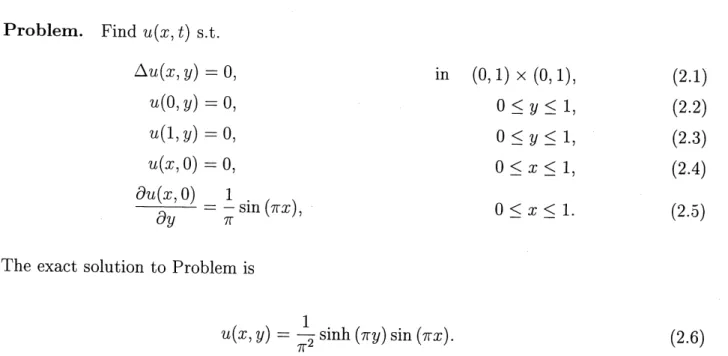
Problem. Find $u(x, t)\mathrm{s}.\mathrm{t}$.

$\triangle u(x, y)=0$, in _{$(0,1)\cross(0,1)$}_, _(2.1)

$u(0, y)=0$, $0\leq y\leq 1$, (2.2)

$u(1, y)=0$, $0\leq y\leq 1$, (2.3)

$u(x, 0)=0$_, $0\leq x\leq 1$, (2.4)

$\frac{\partial u(x,0)}{\partial y}=\frac{1}{\pi}\sin(\pi x)$,

$0\leq x\leq 1$. (2.5)

The exact solution to Problem is

$u(x, y)= \frac{1}{\pi^{2}}\sinh(\pi y)\sin(\pi x)$_. _(2.6)

This is an inverse problem. Usual approaches

are

applications of the regularization and

least square method or $\mathrm{A}\mathrm{I}$. We tried

some

$\mathrm{m}\mathrm{e}\mathrm{t}\mathrm{h}\mathrm{o}\mathrm{d}\mathrm{s}[\mathrm{s}, 8]$, however we were not satisfied.

Here, we apply IPNS directly. We

use

the

same

order approximation in $\mathrm{x}$ and $\mathrm{y}$ directions

for simplicity. $N$ represents the order in spectral collocation method. The number of_total

collocation points is $(N+1)^{2}$. The coefficient matrix of the linear system which is derived

by applying the spectral collocation method is $M\cross M$ matrix, where

$M=N(N-1)$

_. _This

is a sparse matrix but is not a _{band matrix. Fig. 1. shows the form of the coefficient matrix.}

Here, $*\mathrm{r}\mathrm{e}\mathrm{p}\mathrm{r}\mathrm{e}\mathrm{s}\mathrm{e}\mathrm{n}\mathrm{t}_{\mathrm{S}}$

non-zero

element.

$\ovalbox{\tt\small REJECT}*****$ $*****$ $*****$ $*****$ $********$ $********$ $********$ $********$ $********$ $********$ $********$ $********$ $********$ .$********$ $********$ $********$ $********$ $********$ $********$ $********\ovalbox{\tt\small REJECT}$

(3)

In the following chapters, we introduce the results by using various solvers.

3 Gauss

elimination

method

In this section thenumerical results by the Gausselimination method with 120 digit numbers

are shown. The maximum errors, CPU times and the used memory are shown in Table 1.

The amount of operations is proportional to $M^{3}(N^{6})$ and the amount of use of memory is

proportional to $M^{2}(N^{4})$. In this paper, all numerical calculation

are

executed by Compaq

$\mathrm{A}1_{\mathrm{P}}\mathrm{h}\mathrm{a}\mathrm{S}\mathrm{e}\mathrm{r}\mathrm{v}\mathrm{e}\mathrm{r}$ ES40 (CPU : $21264-666\mathrm{M}\mathrm{H}_{\mathrm{Z}}$, memory : $4\mathrm{G}\mathrm{B}$).

Table 1. Numerical results by the Gauss elimination method.

4 SOR method

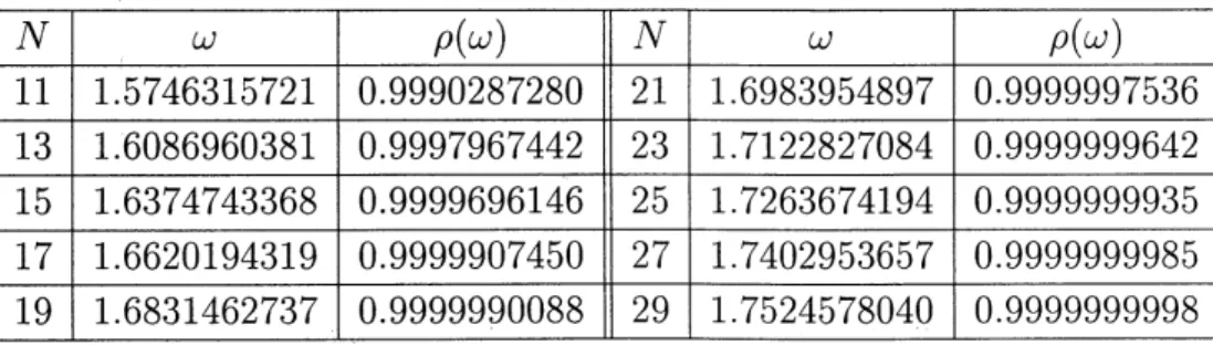
In this section the SORmethod for Cauchy problem is considered. We calculate the optimum

relaxation parameters $\omega$ and the spectral radiuses $\rho(\omega)$ to the iterations matrices of SOR

method by numerically. The results when 10 $\leq N\leq 30$

are

shown in Table 2. When

$N$ is even number, the value of $\omega$ is more than 1. In these case, the SOR method are

not converged. When $N$ is odd number, the spectral radius to the optimum relaxation

parameter is approximately 1. It shows that the convergence of the SOR method is very

slow. Therefore, the SOR method doesn’t suit this problem.

(4)

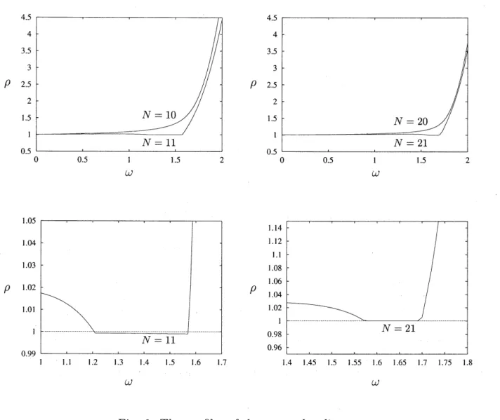
Fig. 2. shows the profiles of the spectral radiuses in $N=10,11,20$ and 21. $\rho$ $\rho$ $\omega$ $\omega$ 1.14 1.12 $\mathrm{l}.\mathrm{l}$ 1.08 1.06 $\rho$ $\rho$ 1.04 1.02 $[$ $0.98$ $0.96$ 1.4 1.45 1.5 1.55 I6 1.65 1.7 1.75 1.8 $\omega$ $\omega$

Fig. 2. The profiles of the spectral radiuses.

5 CGS method

In this section some numerical results by the CGS method are shown.

First, Fig. 3 shows the results obtained with unpreconditioned CGS method. In this

(5)

$,=^{\mathrm{o}\iota}0$

$\sim=^{\mathrm{N}}=$

$\zeta^{\mathrm{e}}$

.

Iteration number

Fig. 3. Unpreconditioned CGS method

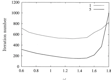
Next, we show the results by PCGS method. The SOR method was used as

precondi-tioner. The iteration step of the SOR method is fixed. The iteration numbers of the CGS

method to the relaxation parameters when the number of iteration for the SOR method are

1 and 5 are shown in Fig. 4. Here, $N=20$ and 60 digit numbers have been used.

Itera-tions were stopped when $||r_{n}||_{2}/||b||_{2}\leq 10^{-60}$. The vertical axis represents the iteration

numbers of the CGS method. The CGS method is converged for various values of the

relax-ation parameter $\omega$. When the relaxation parameter $\omega$ is 1.3\sim 1.4, it seem that the iteration

numbers are least. On the other hand, the SOR method is not converged when $N=20$.

Therefore, the optimal relaxation parameter $\omega$ in original SOR method is not important.

$\omega\succ_{\neg}$

$\Delta\underline{\supset\in\not\supset}$

$.+\overline{\frac{\mathrm{o}}{c6D}}$

$\underline{\dot{+\omega_{\partial}}}$

$\omega$

(6)

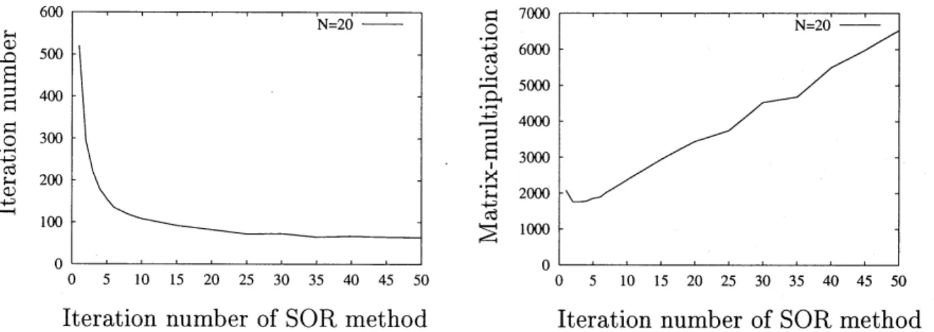
Fig. 5 shows that the iteration number and the amount of operations of the PCGS

method to the iteration step of the SOR method with $\omega=1.3$ and 60 digit numbers.

Iterations

were

stopped when $||r_{n}||_{2}/||b||_{2}\leq 10^{-60}$. The horizontal axis represents the

number ofiterations for SOR method. The vertical axis represents the number of iterations

for CGS method and the number of matrix-multiplications for the CGS method and the

SORmethod in the left figure and right figure, respectively. The mount of operations of the

PCGS is least when the number of iterations for SOR method is 3.

$\overline{\omega}$

$r \frac{\lrcorner\supset\Xi}{\mathrm{E}}$

$.-^{\underline{\Phi}}+\overline{\frac{\mathrm{o}}{-^{6}\mathrm{c}^{\partial}}}$

Iteration number ofSOR method Iteration number of SOR method

Fig. 5. Relationship between CGS and SOR

Fig. 6 shows the convergence behavior ofPCGS method when $N=60$ and digit number

is 400. In preconditioner SORmethod,

we

take the parameter $\omega=1.4$ and fixed the number

of iterations is 3. Iterations

were

stopped when $||r_{n}||_{2}/||b||_{2}\leq 10^{-90}$. In this

case

our

method needs only $300\mathrm{M}\mathrm{B}$ memories, but the Guass elimination method needs $2600\mathrm{M}\mathrm{B}$.

$.=0^{\circ \mathfrak{j}}$

$=\backslash _{\mathrm{N}}=$

$\sigma_{-}^{\mathrm{P}}$

Iteration number

(7)

6 Conclusion

In this paper, the Gauss elimination method, the SOR method and the PCGS method are

applied to the linear system which is derived by IPNS to Cauchy problem. The PCGS

method with the SOR method that iteration step is fixed

as

preconditioner is effective.

The memory could be substantially saved compared with the

case

to have used the Gauss elimination method.

Acknowledgements

This work is partially supported by Grant-in-Aid for Scientific Research$(\mathrm{N}\mathrm{o}. 10354001)$

and by CCSE of Japan Atomic Energy Research Institute.

References

[1] C. Canuto, M. Y. Hussaini, A. Quarteroni, T.A. Zang, Spectral Methods in Fluid Dynamics,

Springer-Verlag, New York, 1988.

[2] H.Han and H. -J. Reinhardt, SomeStability Estimates for Cauchy Problems for Elliptic Equations, J.

Inv. Ill-Posed Problems, 5(5), 1997, pp.1-18.

[3] H. Imai, Application of the Fuzzy Theory and Spectral Collocation Methods to an Ill-Posed Shape

Design Problem With a Free Boundary, in “Inverse Problems in Mechanics,” Eds. S. Saigal and L.G.

Olson, 186, pp.103-107, The American Society of Mechanical Engineers, 1994.

[4] H. Imai and T. Takeuchi, Application of the Infinite-Precision Numerical Simulation to an Inverse

Problem, Proceeding of 1998-WorkshoponMHD Computations “StudyonNumerical Methods Related

toPlasma Confinement”, $\mathrm{N}\mathrm{I}\mathrm{F}\mathrm{S}_{-}\mathrm{p}\mathrm{R}\mathrm{o}\mathrm{c}_{- 40}$, 1999, pp.38-47.

[5] H. Imai, T. Takeuchi and M. Kushida, On Numerical Simulation of Partial Differential Equations in

Infinite Precision, Advances in MathematicalSciences and Applications, 9(2), 1999, pp.1007-1016.

[6] H. Imai, T. Takeuchi, S. S. Shanta and N. Ishimura. On Numerical Computation of Lyapunov

Expo-nents ofAttractorsin Free BoundaryProblems, Proceeding of 1999-Workshopon MHD Computations

“Studyon Numerical Methods Related to Plasma Confinement”, $\mathrm{N}\mathrm{I}\mathrm{F}\mathrm{S}- \mathrm{P}\mathrm{R}\mathrm{o}\mathrm{c}_{-4}6$, 2000, pp.21-29.

[7] D. E. Knuth, The Art _of Computer Programming, Addison-Wesley, 1981.

[8] A. Sasamoto, H. Imai and H. Kawarada, A Practical Method for an Ill-Conditioned Optimal Shape

Design ofa Vessel in Which Plasma Is Confined, in “Inverse Problems in Engineering Sciences”, Eds.

M. Yamaguti et al., pp.120-125, Springer-Verlag, 1991.

[9] S.S.Shanta, T. Takeuchi, H. Imai, M. Kushida, Numerical Computation ofAttractorsinFree Boundary

Problems, Advancesin Mathematical Sciences and Applications, 11(2), 2001. (in press)

[10] D. M. Smith, A FORTRAN Package For Floating-Point Multiple-Precision Arithmetic, Transactions

on Mathematical Software 17, 1991, pp.273-283.

[11] P. Sonneveld, CGS, A Fast Lanczos-type Solver for Nonsymmetric Linear Systems, SIAM J. Sci. Stat.

Comput., 10, 1989, pp.26-52.

[12] Tarmizi, T. Takeuchi, H. Imai, Numerical $\mathrm{S}^{r}\mathrm{i}\mathrm{m}\mathrm{u}\mathrm{l}\mathrm{a}\mathrm{t}\mathrm{i}_{\mathrm{o}\mathrm{n}}$

of One-Dimensional Free Boundary Problems in