DESIGN GUIDELINE OF TREES PLANTING ALONG THE ROADSIDE CONSIDERING IMPACTING OF THE CO2 EMISSION DISPERSION BY VEHICLES

DESIGN GUIDELINE OF TREES PLANTING ALONG THE ROADSIDE CONSIDERING IMPACTING OF THE CO2 EMISSION DISPERSION BY VEHICLES

著者 ヌル アイニ

著者別表示 NURUL AINI journal or

publication title

博士論文本文Full 学位授与番号 13301甲第1924号

学位名 博士（理学）

学位授与年月日 2020‑09‑28

URL http://hdl.handle.net/2297/00061365

Creative Commons : 表示 ‑ 非営利 ‑ 改変禁止 http://creativecommons.org/licenses/by‑nc‑nd/3.0/deed.ja

I

Dissertation

学位論文

DESIGN GUIDELINE OF TREES PLANTING ALONG THE ROADSIDE CONSIDERING IMPACTING OF THE CO2 EMISSION DISPERSION BY

VEHICLES

自動車排出ガスの遮蔽効果を考慮した街路樹のデザインガイドラインに関す る研究

Graduate School of Natural Science and Technology Kanazawa University

金沢大学大学院自然科学研究科

Division

: ENVIRONMENTAL DESIGN

Student ID Number

1724052012 Name

NURUL AINI

Chief Supervisor (

: Prof. ZHENJIANG SHEN

September 2020

II

III

Abstract

This Ph.D. research objective to evaluate the design of trees planting on the roadside in impacting the dispersion of CO

emitted from transportation. This research provides design guidelines of trees planting in urban roadside that can improve air quality.

The result can support urban planners, government, or other stakeholders to solve the decreasing air quality due to CO

emission dispersion. It is important because the high CO

concentration influences human health, whereas the roadside is public space that provided for pedestrians who want to travel. Therefore, Computational Fluid Dynamics (CFD) was used to simulate the spread of CO

and analyze air quality in some design trees planting. The results of the simulation were validated using statistical analysis, which is correlation analysis. So, the result could be justified.

The first research is investigating the CO

dispersion emitted from transportation in the study area with trees planting and without tree planting on the roadside. The result confirms the impact of trees planting on CO

dispersion. This result also shows the CO

concentration in the area around the road.

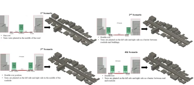
The second research evaluates the row position of trees planting to the road-air quality from CO

emission. The trees planting have some row position that can be implemented on the roadside. Commonly trees area planted in one-row and double row but in a different position. Trees can plant as a one-row position in the middle of the road.

Trees also can plant as double-row positions on both sides of the road as a barrier between road, roadside, and building. This research provides four positions of trees planting. So the result can confirm the best position of trees planting along the roadside in improving air quality that exposed vehicle emission.

On the other side, the trees planting on the roadside not only consider the position of trees planting in improving the air quality, but there is some element design that also influences the CO

dispersion. So, the next research predicts CO

dispersion in different design trees planting patterns. This stage carried out five design of tree planting patterns based on the row position, avenue-tree layout, and space. The result showed the design alternative of tree’s planting pattern that can control air quality from CO

dispersion emitted from motor vehicle.

Keywords: CO

emission, Computational fluid dynamics, trees planting pattern, design

trees planting, air quality.

IV

Acknowledgment

I am very grateful to be a doctoral student at the Urban Planning Laboratory, Kanazawa University. I give my highest appreciation to Prof. Zhenjiang Shen, who has become a kind supervisor for me. Without his guidance and direction, I cannot complete this dissertation easily. I also would like to thank my committee members, Prof. Ito Satoru (Kanazawa University), Prof. Ryoko Ikemoto (Kanazawa University), Prof. Nishino Tatsuya (Kanazawa University) and Prof. Guangwei Huang from Shopia University for their availability in reading my dissertation and providing a detail suggestion for completion of this dissertation.

The last, special acknowledgment is presented for my parents, husband, my lovely

daughter (Zahrany & Harumi chan), and all my friends in Kanazawa and Indonesia that

always support me.

V

Table of Content

Abstract ... III

Acknowledgment ... IV

Table of Content ... V

Table of Figure ... VIII

List of Table ... 10

Table of Equation ... XI Chapter 1. Introduction ... 1

1.1 Research Background ... 1

1.2 Research Purpose and Contribution ... 2

1.3 Literature Review... 3

1.4 Dissertation Organization ... 5

1.4.1 The effect of trees planting on the roadside on the dispersion of CO2 emitted from transportation. ... 5

1.4.2 How positions of trees planting can influence the dispersion of CO2 emission from transportation. ... 6

1.4.3 Impact the design of trees planting patterns on the roadside to the near-road air quality from CO2 dispersion emitted from transportation ... 6

Chapter 2. The effect of trees planting on the roadside on the dispersion of CO

emitted from transportation. ... 7

2.1 Introduction ... 7

2.2 Method ... 8

2.2.1 Study area ... 8

2.2.2 Research framework ... 9

2.2.3 Create the geometry of the study case in 3D modeling. ... 9

2.2.4 Computational domain ... 11

2.2.4.1 Domain size ... 11

VI

2.2.4.2 Boundary Condition ... 11

2.2.5 Fluids mixing analyze ... 12

2.2.5.1 Fluids condition (Air and CO

) ... 12

2.2.5.2 Scalar mixing analysis ... 13

2.2.6 Mesh sizing ... 13

2.2.7 Solving in CFD analysis ... 14

2.3 Result ... 16

2.3.1 Identification the wind speed in the study area ... 16

2.3.2 Identification CO

emission in the study area ... 17

2.3.3 CO

dispersion on the study area in various altitude ... 17

2.3.4 CO

concentration on the road and roadside of the study area ... 19

2.3.5 Similarity analysis ... 21

2.4 Conclusion of chapter 2 ... 24

Chapter 3. How the position of trees planting can influence the road-air quality from CO

emission from transportation ... 26

3.1 Introduction ... 26

3.2 Method ... 27

3.2.1 Research Area ... 27

3.2.2 CO

emission calculation ... 28

3.2.3 Pre-processing in CFD Simulation ... 29

3.2.3.1 The geometry of 3D modeling ... 29

3.2.3.2 Computational domain ... 30

3.2.3.3 Fluid characteristic ... 31

3.2.3.4 Mesh Sizing ... 31

3.2.4 Solving in CFD Simulation ... 32

3.3 Result ... 33

3.3.1 Identification of CO

emission in the research area ... 33

3.3.2 CO

dispersion at various altitude in some position of trees planting pattern 34 3.3.3 Tree’s row position impact on CO

dispersion and CO

concentration. ... 38

3.3.4 The impact of tree’s row position on level air quality ... 39

VII

3.3.5 Validation using similarity analysis ... 41

3.4 Conclusion ... 42

Chapter 4. Design of trees planting pattern: Impacting to the road-air quality for pedestrian from CO2 dispersion emitted from transportation ... 44

4.1 Introduction ... 44

4.2 Method ... 45

4.2.1 Pre-processing in CFD analysis ... 45

4.2.1.1 Build Geometry formation ... 45

4.2.1.2 Determine Computational domain (domain size and boundary condition) 47 4.2.1.3 Assigning the material of 3D modeling ... 49

4.2.1.4 Scalar mixing analysis ... 49

4.2.1.5 Mesh sizing ... 50

3.2.3 Solving in CFD analysis ... 50

4.3 Result ... 52

4.3.1 CO

Emission ... 53

4.3.2 Design of trees planting pattern ... 53

4.3.3 The dispersion of CO

... 55

4.4 Conclusion of chapter 4 ... 58

Chapter 5. Conclusion ... 59

Publication ... 60

Refference ... 61

VIII

Table of Figure

Figure 1.1 The position of trees row (Morakinyo and Lam, 2016). ... 4

Figure 1.2 avenue-tree layouts (Gromke and Blocken, 2015) ... 4

Figure 1. 3 Space of trees planting pattern ... 4

Figure 1. 5 Research framework ... 5

Figure 1. 6 Mesh Sizing in the geometry of modeling ... 14

Figure 2. 1 Orientation of Panglima Sudirman Street as a study case... 9

Figure 2. 2 Research framework of chapter 2 ... 9

Figure 2.3 geometry of 3D modeling a) Trees modeling; b) study area with trees; c) study area without trees ... 10

Figure 2. 4 Domain size in this simulation. ... 11

Figure 2. 5 Boundary condition at study area with trees and without trees ... 12

Figure 2. 6 Wind speed and wind direction recorded by the local weather station in 2017 ... 16

Figure 2. 7 CO

dispersion in the study area with trees planting at different altitude .... 18

Figure 2. 8 CO

dispersion in the study area without trees plating at different altitude . 18 Figure 2. 9 The comparison of CO

dispersion on the study area without trees and with trees. ... 19

Figure 2. 10 CO

concentration in the middle of the road between the area with trees and area without trees ... 20

Figure 2.11 CO

concentration in the right and left of the roadside ... 21

Figure 2. 12 Index of correlation coefficient ... 22

Figure 2. 13 Index of the correlation coefficient ... 41

Figure 3. 1 Location of Research Area ... 27

Figure 3. 2 The position of trees planting in Surabaya city. ... 28

Figure 3. 3 The geometry of 3D modeling. ... 30

Figure 3. 4 Computational Domain ... 31

Figure 3.5 Mesh Sizing ... 32

Figure 3. 6 CO

dispersion at an altitude of 1.8 meter ... 35

Figure 3. 7 CO

dispersion at an altitude of 6 meter ... 36

Figure 3. 8 CO

dispersion at an altitude of 9.6 meter ... 37

IX

Figure 3. 9 Comparison of the dispersion of CO

in every position of trees planting ... 38

Figure 3. 10 The location of the Wall ... 39

Figure 3. 11 The effect of the tree's position to CO2 dispersion... 39

Figure 3. 12 CO

dispersion and CO

concentration on the wall ... 39

Figure 3. 13 Comparison of Level of air quality in every scenario ... 41

Figure 4. 1 Study Area ... 46

Figure 4. 2 Building and tree modeling in the study area ... 47

Figure 4. 3 Domain size and boundary condition ... 48

Figure 4. 4 Mesh sizing for the 3D modeling of the study area ... 50

Figure 4. 5 Trees planting pattern based on the position of trees row ... 54

Figure 4. 6 Trees planting pattern based on the avenue-trees layout in CVF ... 54

Figure 4. 7 Trees planting pattern based on the spacing of the trees ... 55

Figure 4. 8 Five scenarios of trees planting pattern ... 55

Figure 4. 9 CO2 dispersion at an altitude of 1.8 meters in 2D Modelling ... 56

10

List of Table

Table 2. 1 The characteristic of building in the study area ... 10

Table 2. 2 The Characteristics of trees in the Case Study. ... 10

Table 2. 3 Vehicle emission factor ... 13

Table 2. 4 Average daily traffic ... 17

Table 2. 5 CO

emissions in the research area ... 17

Table 2. 6 CO2 dispersion at various altitude ... 22

Table 2. 7 Correlation of CO

dispersion in study area with trees and without trees ... 22

Table 2. 8 CO

concentration at an altitude of 1 meter in various distance of study area ... 23

Table 2. 9 Coefficient correlation of CO

concentration in study area with trees ... 23

Table 2. 10 Coefficient correlation of CO2 concentration in study area without trees .. 23

Table 3. 1 Vehicle emission factor ... 29

Table 3. 2 The daily average of motor-vehicle number ... 34

Table 3. 3 CO2 emission ... 34

Table 3. 4 CO

Dispersion in different position trees planting based on the different altitude of the modeling ... 37

Table 3. 5 Level of air quality ... 40

Table 3. 6 Coefficient correlation of CO

dispersion ... 41

Table 3. 7 Coefficient correlation of Air quality ... 42

Table 4. 1 Vehicle emission factor ... 49

Table 4. 2 CO2 emission in study area ... 53

Table 4. 3 Analysis of CO

dispersion in the different characteristic of trees planting

pattern at an altitude of 1.8 meters ... 56

XI

Table of Equation

Equation 2. 1 ... 12

Equation 2. 2 ... 13

Equation 2. 3 ... 14

Equation 2. 4 ... 15

Equation 2. 6 ... 15

Equation 2. 7 ... 15

Equation 2. 8 ... 15

Equation 2. 9 ... 22

Equation 3. 1 ... 28

Equation 3. 2 ... 31

Equation 3. 3 ... 32

Equation 3. 4 ... 32

Equation 3. 5 ... 32

Equation 3. 6 ... 32

Equation 3. 7 ... 33

Equation 3. 8 ... 33

Equation 3. 9 ... 41

Equation 4. 1 ... 48

Equation 4. 2 ... 49

Equation 4. 3 ... 51

Equation 4. 4 ... 51

Equation 4. 5 ... 51

Equation 4. 6 ... 51

Equation 4. 7 ... 52

Equation 4. 8 ... 52

1

Chapter 1. Introduction

1.1 Research Background

A common problem that is often faced in urban areas is the growing vehicle number.

This condition causes degradation in air quality because it produces CO

emissions from using gasoline and diesel as fuel. The fuel usage in motor vehicle disperse 34% of the total CO

in the air every day (Sullivan et al., 2004; Jie, 2011; EPA, 2016). CO

from transportation spread quickly to the roadside, which is a facility for pedestrians who want to travel in public space that separates from roadway vehicles. But currently, Co2 dispersion that effects road-air quality can harm pedestrians. High CO

concentration can have a devastating effect on human health, such as headaches, sleepiness, stuffy air, stale, poor concentration, loss of attention, increased heart rate, etc. Based on the standard from The Wisconsin Department of health service (2019), good air quality in the outdoor is the air that has a CO

concentration of 0.025%-0.04% (250-400 ppm). Poor air quality is the ambient air that has a CO

level between 0.1%-0.2% (1,000-2,000 ppm). Meanwhile, CO

concentration affects human health at the level 0.2%-0.5% (2,000-5,000 ppm).

Indonesia, as a developing country, has a very rapid increase in the number of motor vehicles. Data from BPS (2016) shows that motor vehicles were increased by 300% since the 2008-2018. This condition makes the air quality worse decrease. Based on that, roadside design can be a solution to these problems. The roadside has some facilities for the pedestrian that can be implemented on that, such as tree planting. Roadside with trees is proven to influence the distribution of vehicle emissions. It because trees have a function as a barrier or windbreaker so that it will affect the CO

dispersion. (Gromke and Ruck, 2010; Šíp and Beneš, 2016; Jeanjean et al., 2015; Brantley and Hagler, 2014) proved that there are differences in CO

distribution in roadside without trees and with trees.

(Gromke and Ruck, 2010; Šíp and Beneš, 2016 indicate that the presence of trees on

the pedestrian way can increase the concentration of emission, while Jeanjean et al., 2015

display the presence of trees can reduce the level of emission—the difference of trees

planting design that analyzed effect to that result. It indicates that the design to create

good road-air quality (Janhäll, 2015). But in reality, the design of trees planting on the

2

roadside ignore this function and just considers to aesthetic value. This condition caused some different trees planting patterns on the roadside in the urban area.

This condition also happens in urban roadside in Indonesia. Trees planting design on the roadside in Indonesia have various patterns. Moreover, tree planting guidelines (Indonesian Ministry Of Public Works, 2012) do not explain the design of tree planting from an environmentally friendly-view at dispersing CO

emissions. So, some roads with high congestion in Indonesia have poor air quality because they do not have a good design in holding the spread of CO

emissions. Surabaya is a metropolitan city that has traffic jam on some roads. Therefore, Panglima Sudirman street in Surabaya City is made to be a study area in this Ph.D. research for planning the design of trees planting on the roadside that have an impact on the CO

dispersion emitted from transportation.

1.2 Research Purpose and Contribution

The design of trees planting on the roadside must consider the effect of CO

dispersion from transportation, especially in urban areas with chronic congestion to improving the air quality. Therefore, this Ph.D. dissertation aims to evaluate the trees planting design on the roadside considering the CO2 dispersion impacting on air quality. This research can contribute to providing the guideline of trees planting design on the roadside from the environmental-friendly view that impacting on the road-air quality. According to the research aims, these following several objectives to be achieved:

1. Investigating the CO

dispersion emitted from transportation in the study area with trees planting and without tree planting on the roadside.

2. Evaluating the row position of trees planting to the road-air quality from CO

emission

3. Evaluating the trees planting pattern on the roadside based on CO

dispersion

In line with research purpose, this study is expected to give a contribution by:

1. Confirm the effect of tree planting on the roadside to the distribution of CO

emitted from transportation. This result can be comparative data of air quality in

a study area with trees and a study area without trees. So, it can show the function

of tree planting to the road-air quality.

3

2. Provide the trees row position that can improve the air quality exposed to the CO

dispersion emitted from transportation.

3. Provide alternative design of trees planting patterns on the roadside that influence CO

dispersion. This design can be applied in roadside that has chronic congestion to improve air quality.

1.3 Literature Review

Trees are planted on the urban roadside with various patterns. Tree planting design is usually adjusted to the beautiful urban roadside, whereas trees have other functions that are no less important. As a result, some design of trees planting is not appropriate with other tree’s functions.

This research focuses on impacting the trees planting to the road-air quality from the dispersion of CO

emission. It will create the roadside with an environmental-friendly view. So that, trees planting on the roadside must consider some design parameters that have an impact on CO

dispersion. It will automatically influence the near-road air quality.

Therefore, this research combines the three-parameters design of trees planting patterns that can affect CO

dispersion. There is the position of trees planting, avenue-tree layouts, and tree spacing. These parameters, according to the related research and theory about trees planting patterns.

The first design parameters of trees planting patterns is the position of the tree row. There are two types of tree row positions, which are double rows and one rows.

Double rows position has trees row in the left and right of the roadside. While one road position only has trees row on one side, which is in the middle of the road, in the windward or leeward of the roadside. The following figure shows the position of trees rows according to the previous research (Morakinyo and Lam, 2016).

The position of trees become one of design parameters in this research because in

the study location was found trees positions that are more diverse than explained in

previous studies.

4

Figure 1.1 The position of trees row (Morakinyo and Lam, 2016).

The next design parameters in this research is avenue-tree layouts. This avenue tree layout influences the CO

concentration (Jian and Zhang, 2018). Gromke and Blocken (2015) display eight scenarios of avenue-tree design in the street. They divide the tree layout based on crown volume fraction (CVF). Trees are planted in the center of the road, which is the one-row position of trees planting. This research considers this parameters and will be combined with other parameters to create the guideline for trees planting design on the roadside to improving the air quality.

Figure 1.2 avenue-tree layouts (Gromke and Blocken, 2015)

The last design parameters of trees planting pattern is space. There is a theory about tree patterns, according to Nursery (1999). This theory divides planting patterns based on tree spacing (column) and row spacing. The type is square, hedgerow, double, and triangle. At the square profile, the distance between rows and between trees is approximately the same. For the Hedgerow pattern, the space between trees in a row is much closer. Meanwhile, in a square planting pattern, the double pattern is interplanting a tree in the center of four trees. The last pattern is a triangle, and all trees are the same distance from each other. Usually, these patterns are used to calculate the number of trees per acre. But this research will be implemented in the urban roadside.

Figure 1. 3 Space of trees planting pattern

5

These three designs parameters will be combined and applied in the trees planting pattern on the roadside to get a better design for improving the air quality from the CO

emission dispersion.

1.4 Dissertation Organization

The main body in this research divided into 4 chapters (Figure 1.5). The first discussion displays investigating the CO

dispersion emitted from transportation in the study area with trees planting and without tree planting on the roadside. The next discussion is evaluating the row position of trees planting to the road-air quality from CO

emission. After that, the next section is predicting the CO

dispersion in different trees planting patterns based on some parameters design. The last discussion is analyzing the crown shape of trees planting on the roadside to improving the air quality.

Figure 1. 4 Research framework

1.4.1 The effect of trees planting on the roadside on the dispersion of CO2 emitted from transportation.

This chapter simulates the CO

dispersion in the real 3D modeling according to

the actual physical condition. It is mean that the characteristic of the trees and buildings

in the study area were built according to reality. This research displays the comparison of

CO

dispersion in the study area without trees and with trees. So, this work confirms the

impact of trees planting on the near-road air quality from the distribution of CO

emitted

6

from transportation. This result can be comparative data of air quality in a study area with trees and a study area without trees.

This chapter has been published on International Review for Spatial Planning and Sustainable Development, Volume 7 Issue 4 Pages 97-112, entitled The Effect of Tree Planting within Roadside Green Space on Dispersion of CO

from Transportation.

1.4.2 How positions of trees planting can influence the dispersion of CO2 emission from transportation.

This section discusses the influence of some design positions of trees planting on dispersing CO

. Some row positions of trees planting can be applied to the urban roadside.

This research found some type of single and double row positions in the study area. It will influence the tree’s ability to dispersing CO

. As a result, some row position is not effective in improving the air quality from the distribution of CO

emission. Therefore, this study evaluates this row position to get the best row position of trees planting in dispersing CO

. So, it can influence optimally to improve near-road air quality. This chapter has been accepted in the International Journal of Sustainable Society.

1.4.3 Impact the design of trees planting patterns on the roadside to the near-road air quality from CO2 dispersion emitted from transportation

This section discusses some design of trees planting patterns to improve the near- road air quality. This chapter displayed five scenarios of trees planting patterns according to some parameters design, which is the position, the avenue-tree layout, and space. So, it can predict the CO

dispersion in different design trees planting patterns. So, it will provide some alternatives design of trees planting patterns on the roadside that influence CO

distribution. This design can be applied in roadside that has chronic congestion to improve air quality.

This chapter has been accepted in the International Journal of Sustainable Society, entitled

Design of trees planting pattern: Impacting on the road-air quality for pedestrians from

CO

dispersion emitted from transportation.

7

Chapter 2. The effect of trees planting on the roadside on the dispersion of CO

emitted from transportation.

2.1 Introduction

The growth of motor vehicles increases rapidly every year in urban areas, especially in developing countries such as in Indonesia. Most of the citizens prefer to use private vehicles than public transportation. The number of motor vehicle increase from 61,685,063 unit in 2008 become 146,858,759 unit in 2018. It causes a lot of congestion in Indonesia, especially in megapolitan and metropolitan cities that have a high population.

This condition has a negative impact on near-road air quality because these vehicles disperse emissions emitted from fuel usage. There is some type of emission from transportation, which is CO

, PM, and NOx. The use of gasoline in vehicles produces more CO

emissions than PM and NOx.

Conversely, traffic with diesel as a fuel can reduce CO

but produce more PM and NO

emissions. But generally, most motorized vehicles in the world use gasoline, and others use diesel (Sullivan et al., 2004; Jie, 2011). According to that, transportation became one of the biggest contributors to CO2 in the world (EPA, 2016).

CO

is a greenhouse gas that has many negative impacts. On a small scale, this gas can easily spread to the roadside located near the road. Roadside is a public facility for pedestrians who want to travel in space that separates from roadway vehicles. According to the location, this area is the space that will be directly affected by the spread of CO

emissions. So. it will be very vulnerable to have poor air quality. Therefore, proper roadside design should be considered to solve this problem.

As is generally known, CO

can spread to the larger area due to airflow, i.e., wind

speed. On the other hand, the tree also has a function as a windbreak. Therefore, trees are

important elements that must be considered on the side of the road. But there are still

many urban roadside Indonesia that does not have trees. Even though, Indonesian

Ministry Of Public Works (2012) in tree planting guidelines on-road network system

suggests that the side of an urban road is better planted with trees. It proved from some

previous research that shows the correlation between trees on the roadside and emission

dispersion. Generally, it was simulated by CFD (Computational Fluid Dynamics), but

there is a different result from this previous research. Research from Gromke and Ruck

8

(2010), Janhäll (2015), and Šíp and Beneš (2016) display that trees can increase the concentration of emission. These studies did not consider the various building height and building layout.

Meanwhile, other research from Jeanjean et al. (2015) proved that trees could reduce ambient levels of road traffic emissions. This research has built modeling based on real buildings with various height and layout on a city scale. However, their study ignored the roadside tree characteristics such as tree trunks and crowns in their simulation models.

Therefore, this study focuses on investigating CO

distribution in a 3D model based on the actual physical condition of the environment. This research creates build and trees in 3D modeling based on the real situation. The result will confirm the effect of tree planting on the distribution of CO

emitted from transportation. It can be comparative data of air quality in a study area with trees and a study area without trees. So, it can show the function of tree planting to the near-road air quality. This research can contribute to providing comparable CO

distribution data on the side of the road planted with trees and without trees in a real physical environment.

2.2 Method 2.2.1 Study area

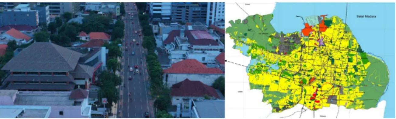
The study area of this research is Panglima Sudirman street in Surabaya city.

Surabaya is geographically located in 07˚09’00 “- 07˚21’00” South Latitude and 112˚36`-

112˚54` East Longitude. Surabaya is a metropolitan city with the most populous city in

Indonesia, which is more than 3 million live there. There were many congestions on

several main roads due to the high number of private vehicles. One of the roads that have

chronic congestions in Surabaya City is Panglima Sudirman street. In peak hours, this

road always has high congestions. The department of transportation in Surabaya city

shows that vehicles number that through this road reached 130508 for 16 hours (Surabaya

City Transportation Department, 2012). Figure 2.1 displays the location of that road in

Surabaya City. This road has a pedestrian on the right and left side. The buildings around

the road have various layout and height. So, this road appropriate to be a case study to

investigate the CO

dispersion.

9

Figure 2. 1 Orientation of Panglima Sudirman Street as a study case

2.2.2 Research framework

This following figure displays the research framework of this chapter. This research focuses on investigating the dispersion of CO2 along the roadside without trees and with trees. The comparison of these two conditions provides the difference CO2 distribution on the side of the road planted with trees and without trees in a real physical environment. Achieving this goal requires several stages of analysis and requires some data to support each analysis. The stages of the analysis process in this study are displayed in the following research framework.

Figure 2. 2 Research framework of chapter 2

2.2.3 Create the geometry of the study case in 3D modeling.

The first stage in this research before simulating is to create the modeling in 3D.

This research uses sim studio tools software to develop geometry. There is some element

that must consider which are trees, pedestrian way, road, and the buildings. These

10

elements were built according to reality. The length of the road that will be developed is 100 meters. The width of the road is 18 meters, and the width of the roadside is 6 meters.

The buildings and the trees built based on the actual conditions. Table 1 shows the characteristic of building in the study area, while Table 2.1 displays the characteristic of the trees in the left and right of the roadside. Based on Table 2.1 and Table 2.2, it can be seen the buildings and the trees have various characteristics. The geometry of this physical condition will create using a sim studio tool, but there is an assumption to create the trees. The canopy will build in the same shape. Then the canopy base height of 1/3 the canopy top height (Gromke and Ruck, 2010; Jeanjean et al., 2015; Šíp and Beneš, 2016).

This research has two modeling to simulate which area study area with trees and study area without the trees. The geometry of this model display in Figure 2.1.

Table 2. 1 The characteristic of building in the study area

Number of Building Width (m) Length (m) Height (m)

1 24 18 12

2 14 30 20

3 20 35 18

4 26 40 16

5 18 40 12

6 40 12 5

7 8 20 10

8 5 5 4

Table 2. 2 The Characteristics of trees in the Case Study.

Trees in The right side Tress in The left side

Diametre of

Trunk Height Diameters Of Canopy

Diametre of

Trunk Height Diameters Of Canopy

50 12 7 60 14 8

50 12 7 50 14 7

20 5 3 50 12 7

20 5 3 50 12 7

20 5 3 60 14 8

30 14 4 50 12 6

40 14 5 40 10 5

50 14 7 40 10 5

50 14 7 50 12 6

Figure 2.3 geometry of 3D modeling a) Trees modeling; b) study area with trees; c) study area

without trees

11

2.2.4 Computational domain

The next step after creating the geometry in 3D modeling is to create the computational domain. The computational domain refers to a simplified form of the physical domain both in terms of geometrical representation in domain size and boundary condition for that domain. This computational domain has to maintain all the important physical features of the problem but can ignore small details (Li, 2008). So, there are two steps in the computational domain, which create the domain size and determine the boundary condition.

2.2.4.1 Domain size

This research creates the size according to the previous research from Franke et al. (2004, 2007). That domain size commonly used for urban research, especially in the street canyon or pedestrian way. Based on that, the inlet and the lateral in urban area simulation should be positioned 5H

from the building. The outflow boundary should be a minimum of 15 H

away from the building. The top boundary at least 5H

away from the building. H

is the size of the tallest building in the modeling. The domain size in this research shows in Figure 2.4.

Figure 2. 4 Domain size in this simulation.

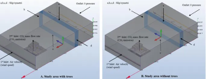
2.2.4.2 Boundary Condition

After creating the domain size, the next step is determining the boundary condition.

There is some part of the boundary in 3D modeling that should be arranged. There are top, lateral, inlet, and outlet. The Inlet surface is the inflow of the fluid. This research has two inlets. The first inlet is the source of wind speed, and the second is the source of CO

emission from transportation. While the inlet surface is an outflow of the simulation, and

0 pressure is assigned in this part. Then, the top and lateral conditions assumed the fluid

12

flow along a wall instead of stopping at the wall. So, the slip/symmetry condition assign on these surfaces. Figure 2.5 displays the boundary condition of this research.

Figure 2. 5 Boundary condition at study area with trees and without trees

2.2.5 Fluids mixing analyze

2.2.5.1 Fluids condition (Air and CO

)

There is two fluid that will simulate in this research, which is air and CO

. Air and CO2 have different density. The density of air (𝜌

) is 1.2047 e-6 g/mm

, and density of carbon dioxide (𝜌

) is 1.773e-6 g/mm

. Air and CO

in the modeling need velocity to make fluids flow, so air velocity and mass flow rate of CO

is needed. Air can move in modeling if there is a velocity that is coming from wind speed. While the mass flow rate of CO

comes from CO

emission.

The data of wind speed is taken from Local Weather station (Indonesia Meteorology Climatology and Geophysics Council, 2019). Meanwhile, the value of the mass flow rate can be calculated using the CO

emission equation (AEA, 2012; Hidayat, 2013).

Equation 2. 1

Based on that equation, we should know the vehicle number per hour in the street,

length of the street in modeling, and emission factor. This number vehicle obtained

through a direct survey at the study location during peak hours. Peak Hours in the research

area occur three times a day, which is in the morning, noon, and afternoon. The survey

was conducted starting at 7-8 am in the morning, at 12 am – 1 pm at noon and at 6-7 pm

in the afternoon for two days, which is on weekday and weekend. The next data that we

13

need is the length of the street. This study uses 100 meters to simulate the study case.

Whereas this equation also needs an emission factor of transportation for calculating this research, Then this research use standard of Vehicle classification according to (AEA, 2012). Table 2.3 shows the standard of emission factor.

Table 2. 3 Vehicle emission factor Transportation

classification

Definition Average emissions

(kgCO

/km) Small car Small petrol car, up to the 1.4-liter engine 0.16442 Medium car Medium diesel car, from 1.7 to 2.0 liter 0.17573 Large Car Large diesel car, over 2.0 litre 0.23381 Motorcycle Small petrol motorbike (mopeds/scooters) 0.08499

2.2.5.2 Scalar mixing analysis

The important step in this research is mixing the air and CO

. As explained before, these fluids have different density, so scalar mixing analysis is needed to know the fluid dispersion after mixing. The following equation is used to analyze the scalar mixing where 𝐴 is air and display in scalar 0, while 𝐵 is CO

and shows in scalar 1.

Equation 2. 2

𝐽

is the mass flux of air. This is how much air is transferred (per time and unit area normal to the transfer direction). It is proportional to the mixture mass density (𝜌

). The density of air (𝜌

) is 1.2047 e-6 g/mm

, and the density of carbon dioxide (𝜌

) is 1.773e- 6 g/mm

. D

is the diffusion of scalar quantities based on Fick’s Law. The diffusion coefficient to mixing air and CO

is 0.16 cm

/s. The units of the Diffusivity coefficient are length squared per time. This simulation uses 3D modeling, so to get 𝐽

is proportional to the gradient (▽)of the species mass fraction (𝑚

).

2.2.6 Mesh sizing

This part is the last stage for pre-processing in CFD analysis. This part has divided the geometry of 3D modeling become a small shape, which is the element and node.

Element is small pieces from geometry, and the node is a corner of each element. The

nodes and elements make up the mesh. Mesh is needed in computational simulation to

make the computer easy for the mathematical calculation in CFD analysis. There are

14

many shapes of mesh that we can use. This research uses tetrahedral shape because this shape is appropriately used in 3D modeling.

Figure 1. 5 Mesh Sizing in the geometry of modeling

2.2.7 Solving in CFD analysis

This part is a simulation part using CFD to get the result of CO2 dispersion in the study area. The airflow and co2 flow will be simulated, and this fluid will be mixing, so it can be known the air quality because of co2 dispersion in the study area. Therefore, some equation for CFD is needed to start the simulation. This research uses the Navier- Stokes equations (NSE) to describe the movements of fluids, which are air and CO2.

This research has some assumptions to simulate these fluid flow. Air moves in steady condition and not compressed (incompressible) or density (𝜌) constant. The wind direction in the environment is considered unidirectional during the simulation. This airflow uses turbulent because this simulation wants to analyze the airflow and CO2 dispersion in two study cases with different physical environments. Then, this simulation just considers the airflow, so the parameters used are only related to airflow boundary does not heat transfer boundary.

Accordingly, some equation is needed to analyze a concentration gradient in the species. The following equation is used for the conservation of mass is (Equation 2.3).

Equation 2.

3

Where:

𝜕𝜌

𝜕_𝑡

is the partial derivative of 𝜌 with respect to 𝑡 𝜌 is density

𝑡 is time

The tensor gradient (∇) is the stress variable.

𝑢 is the flow velocity

∇𝑢 spatial derivatives of the flow velocity

15

Then the conservation of momentum based on Navier-Stokes Equations in 3D modeling using the following formula.

Equation 2. 4

Equation 2. 5

Equation 2. 6

The Navier–Stokes equations have limitations for describing turbulent flows, which is the time-averaged RANS equation. The limitation is the introduction of the Reynolds stress term, which accounts for turbulent fluctuations. Hence, the K-ϵ model equation is used for turbulent kinetic energy used to support this CFD analysis. There is a two-equation. The first transported variable is the turbulent kinetic energy (k). The second transported variable is the rate of dissipation of turbulent kinetic energy (ε).

Equation 2. 7

Equation 2. 8

Where ꭒ is the fluid velocity ( 𝑚 𝑠

) , 𝜌 is the fluid density (𝑘𝑔 𝑚

), i represent x.Then, j represents x,y, and z (coordinate geometry in boundary). 𝐸

is the component of the rate of deformation. 𝑢

represents the velocity component in the corresponding direction. 𝜇

represents turbulent viscosity which is 𝜇

= 𝜌𝐶

𝜀

.

16

Accordingly, the equation has some standard constant that should be divided. There are 𝜎

, 𝜎

, 𝐶

, 𝐶

and 𝐶

. The value of standard constants are the following:

2.3 Result

2.3.1 Identification the wind speed in the study area

This research chooses one of the roads in Surabaya city as a study case. Surabaya city as a tropical city has only two seasons, which are dry and rainy seasons. The dry season occurs from April-September when monthly rainfall is below 60 mm. The dry season occurs from April-September when monthly rain is more than 60 mm. But the climate change influence this time season. In 2017, the rainy season was longer than the dry season. This season occurs in November-June, whereas the dry season occurs in July- October. This condition influences the wind speed in this city.

The following figure shows the wind speed in 2017 in the study area. According to that figure, the average wind speed in 2017 is 1.6 knots, whereas the highest wind speed is 10 knots. This simulation uses 10 knots or 5.14 m/s of wind speed as a source of air velocity, which is 1

inlet (inflow) of fluids in this analysis.

Figure 2. 6 Wind speed and wind direction recorded by the local weather station in 2017

17

2.3.2 Identification CO

emission in the study area

This part explains the calculation of CO

emission, and it will be used as a 2

inlet (mass flow rate of CO

) in the simulation. Table 2.4 shows the average number of vehicles per hour obtained by a survey in the study location. Then table 2,5 shows the calculation of CO

emission.

Table 2. 4 Average daily traffic

Classification type of motor vehicle Total (unit/hour)

Small car Private car 2050

Small car Public Transportation 111

Medium car Mini Bus 233

Medium car Pick Up / Box 1

Medium car Mini Trucks 166

Large car Big bus 3

Large car Truck 2 axis 1

Large car Truk 3 axis 1

Motorcycle Motorcycle 6814

TOTAL 9380

Table 2. 5 CO

emissions in the research area

Transportation type

Average daily traffic(unit/hour)

Length of the street (km)

Emission factor

CO2 emission (kg/hour)

Small car 2161 0.1 0.16442 35.5

Medium car 400 0.1 0.17573 7.0

Large car 5 0.1 0.23381 0.1

Motorcycle 6814 0.1 0.08499 57.9

TOTAL 100.6

Based on that result, the number of motorcycles is the highest than other transportation classification, so CO

emitted from the motorcycle reaches 57.9 kg/hour. Meanwhile, the total CO

emission in one hour is 100.6 kg/hour. This emission is determined as the mass flow rate of CO

emission in this simulation.

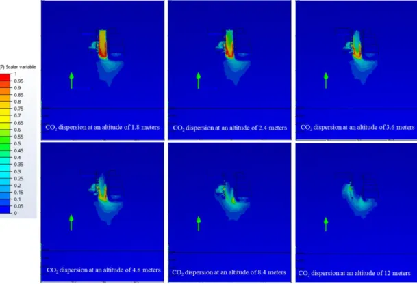
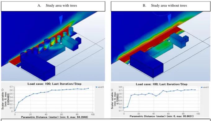
2.3.3 CO

dispersion on the study area in various altitude

This section appearance the distribution of CO

in the study area. Figure 2.7 and Figure 2.8 show the Dispersion of CO

at different elevations which is at 1.8 meters until 12 meters. In every altitude, there are differences in CO

dispersion between modeling with trees and modeling without trees. Scalar variable shows the percentage of CO

dispersion in the study area. Based on the color of the scalar in the following figure, the scalar of CO

in the study area without trees is higher than the study area without trees.

Moreover, CO

in the study area without trees is more spread out than the study area with

trees.

18

Figure 2. 7 CO

dispersion in the study area with trees planting at different altitude

Figure 2. 8 CO

dispersion in the study area without trees plating at different altitude

19

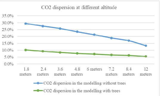
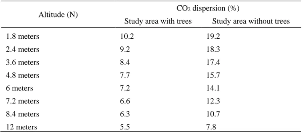
The value of CO

distribution can be seen more clearly in Figure 2.9. This figure shows the comparison of CO

dispersion by percentage at several heights in both models.

Based on that, the model with trees has a higher distribution value. At the height of 1.8 meters, the CO

distribution in the study area without trees is 19.2%%. While CO

spread by10.2% in the modeling with trees, this result shows that trees in the roadside can decrease CO

dispersion by 9% at an altitude of 1.8 meters. It is also displayed in another different height.

Figure 2. 9 The comparison of CO

dispersion on the study area without trees and with trees.

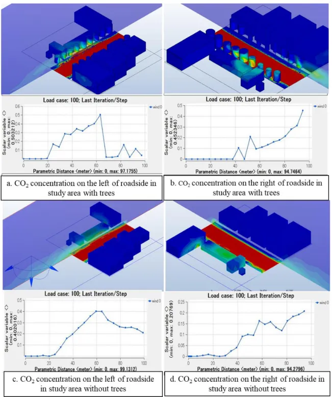
2.3.4 CO

concentration on the road and roadside of the study area

This part will compare the CO

dispersion between the roadside with trees and roadside without trees. The CO

dispersion on the roadside shows a different result because it has various characteristics of building around the roadside. On the right side, it has higher buildings than on the left side so that it will influence the result of CO

dispersion on both sides. Figure 2.10 displays the CO

concentration in the middle of the road. The graphic shows the CO

concentration on the road in the study area without trees and with trees—the result based on the CO

concentration at an altitude of 1.8 meters.

Accordingly, the range of CO

concentration in the road of the study area with trees starts

from 0-0.68% (0-6800 ppm). While 0.2-0.72% (2000-7200 ppm) disperse on the road of

20

study area without trees, it is mean that that study area with trees can decrease the concentration of CO

in the road.

Figure 2. 10 CO

concentration in the middle of the road between the area with trees and area without trees

Another result also shows in Figure 2.11. This figure shows the CO

concentration in the left and right of the roadside. In the study area with trees, a range of CO2 concentrations in the left of the roadside start form 0-0.51 (0-5100 ppm), and CO2 concentration in the right of roadside start from 0-0.48 (0-4800 ppm). In the study area without trees, Co2 concentration has range 0-0.4 (0-4000 ppm) on the left side and 0-0.21 (0-2100 ppm) on the right side. This result indicates that the study area with trees has a higher Co2 concentration than the area without trees.

Accordingly, CO2 concentration in some parts of the study area shows the difference result. So the next part of this research will validate this result to justify the result of this simulation.

A. Study area with trees

CO2 concentration in the middle of the road at an altitude 1 m

B. Study area without trees

21

Figure 2.11 CO

concentration in the right and left of the roadside

2.3.5 Similarity analysis

Based on the result of CO

dispersion at different altitudes and CO

concentrations

in the study area, the validation stage is needed to justify that result. This part uses

correlation coefficient analyses to describe the similarity of the result in the study area

22

without trees and with trees. The value of the correlation coefficient has a range between -1 until +1. The values close to 1 and -1 have very strong correlations, while values close to 0 have weak correlation (Figure 2.12). This values is obtained using equation 2.9. This research uses SPSS software to calculate correlation analyses.

Figure 2. 12 Index of correlation coefficient

Equation 2. 9

Where 𝜌

is the correlation coefficient based on Pearson product moment.

𝐶𝑜𝑣 (𝑥, 𝑦) is the covariance of variable x and y, and 𝜎 is the standard deviation. The first stage is to analyses the similarity of CO

dispersion in study area without trees and without tree. This stage uses 8 data (N) of CO

dispersion in different altitude (Table 2.6), which is 1.8 meters until 12 meters. The result shows in Table 2.7, where the correlation coefficient is 0.965.

The value of coefficient correlation indicates that the CO

dispersion between study area with trees and without trees study have strong correlation. It indicates that differences of physical environment condition at various heights do not affect the distribution of CO

in both study area. So, it can be justified that trees can decrease CO

dispersion.

Table 2. 6 CO2 dispersion at various altitude

Altitude (N) CO2 dispersion (%)

Study area with trees Study area without trees

1.8 meters 10.2 19.2

2.4 meters 9.2 18.3

3.6 meters 8.4 17.4

4.8 meters 7.7 15.7

6 meters 7.2 14.1

7.2 meters 6.6 12.3

8.4 meters 6.3 10.7

12 meters 5.5 7.8

Table 2. 7 Correlation of CO2 dispersion in study area with trees and without trees

𝜌

𝜎𝑥𝜎𝑦

23

CO2 dispersion in the study area

with trees at different altitude

CO2 dispersion in the study area without trees at different

altitude

CO2 dispersion in the study area with trees at different altitude

Pearson Correlation 1 ,965^**

N 8 8

CO2 dispersion in the study area without trees at different altitude

Pearson Correlation ,965^** 1

N 8 8

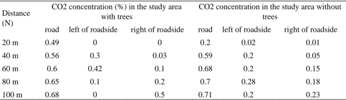
Meanwhile, table 2.8 shows the CO

concentration in the study area of this research. This step will analyze the similarity of that CO

concentration on the road and roadside in both study area, which is study area with trees and without trees. N refers to number of sample of CO

concentration. This research use five sample of CO

concentration in different distance of study area.

Table 2. 8 CO2 concentration at an altitude of 1 meter in various distance of study area Distance

(N)

CO2 concentration (%) in the study area with trees

CO2 concentration in the study area without trees

road left of roadside right of roadside road left of roadside right of roadside

20 m 0.49 0 0 0.2 0.02 0.01

40 m 0.56 0.3 0.03 0.59 0.2 0.05

60 m 0.6 0.42 0.1 0.68 0.2 0.15

80 m 0.65 0.1 0.2 0.7 0.28 0.18

100 m 0.68 0 0.5 0.71 0.2 0.23

Table 2. 9 Coefficient correlation of CO2 concentration in study area with trees CO2 concentration

on the road

CO2 concentration on the left side

CO2 concentration on the right side

CO2 concentration on the road Pearson Correlation 1 -.066 .860

Sig. (2-tailed) .916 .062

N 5 5 5

CO2 concentration on the left side Pearson Correlation -.066 1 -.428

Sig. (2-tailed) .916 .472

N 5 5 5

CO2 concentration on the righ tside

Pearson Correlation .860 -.428 1

Sig. (2-tailed) .062 .472

N 5 5 5

Table 2. 10 Coefficient correlation of CO2 concentration in study area without trees CO2 concentration

on the road

CO2 concentration on the left side

CO2 concentration on the righ tside

CO2 concentration on the road Pearson Correlation 1 .939^* .832

Sig. (2-tailed) .018 .080

N 5 5 5

CO2 concentration on the left side Pearson Correlation .939^* 1 .712

24

Sig. (2-tailed) .018 .177

N 5 5 5

CO2 concentration on the right side

Pearson Correlation .832 .712 1

Sig. (2-tailed) .080 .177

N 5 5 5

*. Correlation is significant at the 0.05 level (2-tailed).

Based on this result, the coefficient correlation of CO

concentration in the study area with trees shows the various result. CO

concentration has a strong correlation between the right side and the road. But it has a weak and very weak correlation between the left side and road, the left side and right side. On the other side, the coefficient correlation in the study area without trees show a strong correlation among CO

concentration in the road, left side, and right side.

Based on that similarity analysis, CO

concentration in the study area can change according to the physical condition, such as trees planting conditions. Hence, it is important to observe in detail the tree planting design to reduce the increase in CO

concentration around the road.

2.4 Conclusion of chapter 2

This research evaluates the CO2 dispersion in the study area with trees and without trees. There are some conclusions from this research. The first conclusion that study area with trees can decrease CO2 dispersion at many different altitudes. The value of CO2 dispersion in the study area with trees is lower than the area without trees. In the altitude 1.8 meters, trees can disperse 9% (9000 ppm) of CO2, while area without trees can distribute CO2 emission by 19.2% (19200 ppm). This result is supported by the validation analysis using correlation analysis. The coefficient correlation is 0.965, which is a strong correlation. So, it can be justified that trees can decrease CO2 dispersion. So, it is important to plant the trees on the roadside to decreasing CO2 dispersion in the air.

Meanwhile, there are differences in the conclusion of CO2 concentration on the

road and roadside. The study area with trees indicates the lower CO2 concentration on

the road than the study area without the tree. But, the study area with trees indicates higher

CO2 concentration on the roadside than study area without trees. The validation process

in the study area without trees shows a strong correlation. It is mean that CO2

concentration on the road, left side, and the right side has similarities of concentration in

the various distance.

25

Meanwhile, CO2 concentration in the study area with trees shows a weak correlation.

CO2 concentration on the left of the roadside has a weak correlation with CO2

concentration on the road and right side. It's mean that the value of CO2 concentration in

the road, left side and right side have low similarity in various distance. It indicates that

CO2 concentration can change according to the physical condition, such as trees planting

conditions. So, this validation proves that planting trees does not always increase

concentration on the side of the road and decrease concentration on the road. Hence, it is

important to observe in detail the tree planting design to reduce the increase in CO2

concentration around the road.

26

Chapter 3. How the position of trees planting can influence the road-air quality from CO

emission from transportation

3.1 Introduction

This research focuses on analyzing the impact of the position of trees planting on the CO

dispersion to be consideration trees planting guidelines from an environmental- friendly view. The tree is an essential element in the design of the urban roadside. Trees planted on the roadside are not only for an urban aesthetic but also can give some advantage to the pedestrian because it can control the quality of the environment.

It is common knowledge that urban air quality is getting worse because of the increasing number of motorized vehicles. Gasoline and diesel as fuel usage for the motor vehicle are the primary CO

source in the air. The high CO

concentrations can give disadvantage to environmental quality. It can indicate poor air quality in the area, and it is not suitable for human health. The Wisconsin Department of health service (2019) showed that 0.1%-0.2% (1,000-2,000 ppm) of CO

concentration indicates poor air quality. Meanwhile, it can influence human health in the CO

level by 0.2%-0.5% (2,000- 5,000 ppm).

Therefore, the existence of the tree on the roadside be a solver for that problem. Trees can influence the emission concentration emitted from transportation (Gromke and Ruck, 2010; Šíp and Beneš, 2016; Jeanjean et al., 2015). Roadside with trees proved can decrease the CO

concentration (Jeanjean et al., 2015; Aini and Shen, 2019). There is some position of trees planting on the roadside. (Morakinyo and Lam, 2016) divide the location of trees planting based on the number of the trees row, which is a double row and one row. Double row position shows that trees are planted on the left and right of roadside, while one row commonly plans the trees in the middle of the road.

In reality, there is some position of the trees row that can be found on the road.

Surabaya city, as a study case in this research, has some position of the trees planting. It

because there is no detailed guideline for the position of the trees planting that considers

air quality for environmental-friendly view. Whereas, the position of the tree is very

important so that the road that is passed by the pedestrian can have good air quality.

27

3.2 Method

3.2.1 Research Area

The research area for this study is Surabaya City in Indonesia. Surabaya, as a metropolitan city, has some roads which chronic congestion. This study chooses the road, namely Panglima Sudirman (Figure 3.1), as a road with high traffic jams. In this road, the researcher conducted the observation to calculate the number of the motor vehicle.

This value will be used as basic data to calculate the amount of CO

emissions that will be simulated in this study. This research also creates the physical environment according to the real condition of this research area. There is the road, roadside, and the building.

This study chooses 400 km of road as a study area with various building height and building layout. The wide of the road is 18 m, and the wide of the roadside is 6 m.

Meanwhile, for the position of the trees, this study considers some trees planting position in some road of Surabaya City. Figure 3.2 shows the location of the trees planting that will simulate in this research. There is four research area based on different trees planting pattern. So, it will be known which position of the trees that have the biggest impact in the dispersing of CO

emitted from transportation.

Figure 3. 1 Location of Research Area

28

Figure 3. 2 The position of trees planting in Surabaya city.

3.2.2 CO

emission calculation

This study can be counted using a CO

emission analysis. The following equation will be used to get the total CO

emission from transportation while one hour (AEA, 2012;

Hidayat, 2013).

Equation 3. 1

29

The CO

emission from that equation will be used in the simulation as CO

sources in the mass flow rate. There are some data that we must prepare before calculation. The first data is the volume of the vehicle. This data gets from a survey that already done in the study area. The observation was done three times a day in the weekday and weekend.

Three times show the peak hour in the study area, which is in the morning, noon, and afternoon. The second data is the length of the road that wants to analyze. Then the last data is the emission factor. This emission factor has a different value according to the classification of transportation. This following table shows the emission factor used in this research (AEA, 2012)

Table 3. 1 Vehicle emission factor Transportation

classification

Definition Average emissions

(kgCO

/km) Small car Small petrol car, up to the 1.4-liter engine 0.16442 Medium car Medium diesel car, from 1.7 to 2.0 liter 0.17573 Large Car Large diesel car, over 2.0 liter 0.23381 Motorcycle Small petrol motorbike (mopeds/scooters) 0.08499

3.2.3 Pre-processing in CFD Simulation

The next step for the simulation is pre-processing. There are some stages in this part and will be explained in the following section.

3.2.3.1 The geometry of 3D modeling

According to the position of trees row, this study creates four geometry of 3D

modeling. These models were built using sim studio tools from Autodesk. 1

scenario has

a one-row position, and trees are planted in the middle of the road. 2

scenario is the

double-row position. The trees are planted in both of roadside as a barrier between

roadside and building. 3

scenario also has a double-row position. Trees are planted in

the middle of the roadside. Then the last scenario has a double row position that trees are

planted as a barrier between road and roadside.

30

Figure 3. 3 The geometry of 3D modeling.

3.2.3.2 Computational domain

The computational domain is made simple the physical domain both in the form of geometrical representation in domain size and boundary condition for that domain.

Hence, this part will maintain all of the important physical features of the problem but can ignore small details (Li, 2008).

The first step in the computational domain is determining the domain size. This research use domain size according to the previous study by Franke et al. (2004, 2007). This domain is appropriate to use in urban studies, especially in the street canyon. Based on that domain size, the inlet and the lateral in urban area simulation have to positioned 5Hmax from the building. The outflow boundary should be a minimum of 15 Hmax away from the building. The top boundary at least 5Hmax away from the building. Hmax is the size of the tallest building in the modeling. Domain size in this research shows in Figure 3.4

The second step in the computational domain is assigning the boundary condition.

There are the inlet, outlet, lateral, and top boundary. For the top and lateral conditions, it

will be assigned as the slip/symmetry boundary. It will cause the fluid to flow along a

wall instead of stopping at the wall. It typically occurs along a wall. Then outflow/outlet

condition is a static pressure with a value of 0. Then the last surface is the inlet. The inlet

of this research comes from 2 sources, which are the source of wind and CO

(Figure 3.4)