Vassiliev knot invariants derived from cable Γ-polynomials

Vassiliev knot invariants derived from cable Γ-polynomials

Hideo TAKIOKA (Kyoto University)

Abstract

For coprime integers p(> 0) and q, the (p, q)-cable Γ-polynomial of a knot K is the Γ-polynomial of the (p, q)-cable knot of K, where the Γ-polynomial is the common zeroth coefficient polynomial of the HOMFLYPT and Kauff- man polynomials. In this paper, we give some results on Vassiliev knot invariants derived from cable Γ-polynomials.

1. Introduction

We focus on the zeroth coefficient HOMFLYPT polynomial P

(= F

= Γ) (see the relation (1) in Section 2) and its (p, q)-cabling (P

)

for coprime integers p(> 0), q, which is called the (P

)

-polynomial, the (p, q)-cable Γ-polynomial, etc. It is known that there exists a pair of genus two mutant knots such that their colored Jones polyno- mials coincide for all colors and their P

-polynomials differ [9]. Moreover, for infinitely many Kanenobu knots, their HOMFLYPT polynomials coincide and their (P

)

- polynomials are all different [14]. However, it is known that there exist infinitely many knots with the trivial (P

)

-polynomial [16] and the (P

)

-polynomial is invariant under mutation for any coprime integers p(> 0) and q [4, 15]. In this paper, we consider Vassiliev knot invariants [2, 17] derived from (P

)

-polynomials.

In Section 2, we recall the HOMFLYPT and Kauffman polynomials and their co- efficient polynomials. In Section 3, we recall Vassiliev knot invariants. In Section 4, we consider cabling for knot invariants and Vassiliev knot invariants. In Section 5, we give some results on Vassiliev knot invariants derived from (P

)

-polynomials.

2. The HOMFLYPT and Kauffman polynomials and their co- efficient polynomials

The HOMFLYPT polynomial P (L) = P (L; t, z) ∈ Z [t

, z

] [3, 11]   and the Kauff- man polynomial F (L) = F (L; a, z) ∈ Z [a

, z

] [6] are invariants for oriented links in S

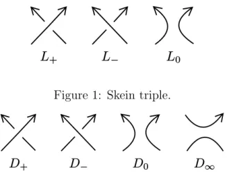
, which satisfy the following skein relations. For the trivial knot U , we have P (U) = F (U ) = 1. For a triple (L

, L

, L

) of oriented links which are identical except near one point as shown in Figure 1, we have

t

P (L

) − tP (L

) = zP (L

).

For a quadruple (D

, D

, D

, D

) of oriented link diagrams which are identical except near one point as shown in Figure 2, we have

aF (D

) + a

F (D

) = z

F (D

) + a

F (D

)

,

This work was supported by KAKENHI (19J00076).

2010 Mathematics Subject Classification: 57M25, 57M27.

Keywords: Alexander-Conway polynomial, Γ-polynomial, HOMFLYPT polynomial, Kauffman poly- nomial, Vassiliev invariant, cable knot.

∗

e-mail: [email protected]

web: https://researchmap.jp/takioka/

Figure 1: Skein triple.

Figure 2: Skein quadruple.

where 2ν = w(D

) − w(D

) − 1 and w(D

), w(D

) are the writhes of D

, D

, respectively.

Let L be an oriented r-component link. The HOMFLYPT and Kauffman polyno- mials are written by the following form:

P (L) = ( − t

z)

X

i≥0

P

(L; t)z

, F (L) = (az )

X

i≥0

F

(L; a)z

,

where P

(L; t) ∈ Z [t

] and F

(L; a) ∈ Z [a

] and they are called the 2ith coefficient HOMFLYPT polynomial and the ith coefficient Kauffman polynomial, respectively. It is known that P

(L; t) = F

(L; √

− 1t

) [8]. Moreover, the polynomial P

(L; t) is a Laurent polynomial in t

. Putting t

= x, we call it the Γ-polynomial Γ(L; x) ∈ Z [x

], that is,

Γ(L; t

) = P

(L; t) = F

(L; √

− 1t

). (1)

3. Vassiliev knot invariants

A singular knot is an oriented immersed circle in S

whose singularities are only trans- verse double points. We assume that each double point on a singular knot is a rigid vertex. Let v be an invariant for oriented knots in S

, which takes values in Q . Then v can be uniquely extended to a singular knot invariant by the Vassiliev skein relation:

v(K

) = v(K

) − v(K

),

where K

is a singular knot with a double point × and K

, K

are singular knots obtained from K

by replacing × by a positive crossing and a negative crossing, re- spectively, as shown in Figure 3. We call v a Vassiliev knot invariant of order d if there exists an integer d such that v(K

) = 0 for any singular knot K

with more than d double points and v(K

) ̸ = 0 for a singular knot K

with d double points. The set of all Vassiliev knot invariants of order ≤ d forms a vector space over Q , which is denoted by V

. There exists a filtration

V

⊂ V

⊂ V

⊂ · · · ⊂ V

⊂ · · ·

Figure 3: Vassiliev skein triple.

in the entire space of Vassiliev knot invariants. Each V

is finite-dimensional. In particular, we have V

= V

=< 1 >. Moreover, we have the following theorem.

Theorem 3.1 ([5]) Let a

be the 2ith coefficient of the Alexander-Conway polyno- mial ∇

(z)(= P (K; 1, z)). Let P

be the 2ith coefficient HOMFLYPT polynomial and P

(1) the dth derivative of P

at t = 1. Let F

be the ith coefficient Kauffman poly- nomial and F

( √

− 1) the dth derivative of F

at a = √

− 1. Then we have a basis of V

for 2 ≤ d ≤ 6 as follows:

V

= < 1, a

> .

V

= < 1, a

, P

(1) > .

V

= < 1, a

, P

(1), a

, a

, P

(1) > .

V

= < 1, a

, P

(1), a

, a

, P

(1), a

P

(1), P

(1), P

(1), F

( √

− 1)/ √

− 1 > . V

= < 1, a

, P

(1), a

, a

, P

(1), a

P

(1), P

(1), P

(1), F

( √

− 1)/ √

− 1, a

, a

a

, a

P

(1), P

(1)

, P

(1), P

(1), a

, F

( √

− 1), F

( √

− 1) > .

4. Cabling for knot invariants and Vassiliev knot invariants

Let p(> 0), q be coprime integers. Let K be a knot and N (K) a tubular neighborhood of K. Let K

be the (p, q)-cable knot of K , that is, an essential loop in ∂N (K) with [K

] = p[l] + q[m] in H

(∂N (K); Z ), where (m, l) is a meridian-longitude pair of K.

We assume that lk(K ∪ l) = 0 and lk(K ∪ m) = +1, where lk is the linking number.

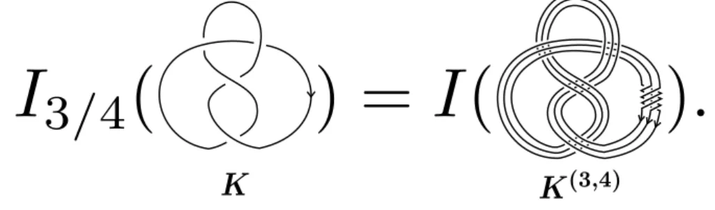
Let I be a knot invariant. The map sending a knot K to the value I(K

) is also a knot invariant, which is called the (p, q)-cabling of I denoted by I

. For example, see Figure 4. If v is a Vassiliev knot invariant of order d, then the (p, q)-cabling v

Figure 4: The (3, 4)-cabling I

of a knot invariant I.

is also a Vassiliev knot invariant of order ≤ d [1, 12]. Since P

(1) is a Vassiliev knot

invariant of order d, (P

)

(1) is a Vassiliev knot invariant of order ≤ d. In this paper,

we consider (P

)

(1) for 1 ≤ d ≤ 6 and 1 ≤ n ≤ 7. By using Kodama’s program

“KNOT” [7], we can calculate (P

)

(K) with 1 ≤ n ≤ 7 for a knot K with small crossings.

5. Vassiliev knot invariants derived from (P ₀ ) _p/q

5.1. Vector space V

We obtain data in Table 1.

P

(1) = − 8a

(P

)

(1) = − 32a

(P

)

(1) = 4P

(1) (P

)

(1) = − 72a

(P

)

(1) = 9P

(1) (P

)

(1) = − 128a

(P

)

(1) = 16P

(1) (P

)

(1) = − 200a

(P

)

(1) = 25P

(1) (P

)

(1) = − 288a

(P

)

(1) = 36P

(1) (P

)

(1) = − 392a

(P

)

(1) = 49P

(1)

Table 1: V

=< 1, a

>

Proposition 5.1

(P

)

(1) = n

P

(1).

Proof. Let ∆

(t) be the normalized Alexander polynomial of a knot K, which satisfies

∆

(t) = ∇

(t

− t

). Then we have ∆

(1) = 0 and ∆

(1) = 2a

(K). By using satellite formula, we have ∆

(t) = ∆

(t

) for the (n, 1)-cable knot K

of a knot K and any n( ≥ 1). Therefore, we have

a

(K

) = (1/2)∆

(1) = (1/2)∆

(t

)

t=1

= (1/2)n

∆

(1) = n

a

(K).

By P

(K; 1) = − 8a

(K) for any knot K, we have

(P

)

(K ; 1) = P

(K

; 1) = n

P

(K; 1).

□ 5.2. Vector space V

We obtain data in Table 2.

(P

)

(1) = − 48a

+ 4P

(1) (P

)

(1) = 6P

(1) + 4P

(1) (P

)

(1) = − 192a

+ 9P

(1) (P

)

(1) = 24P

(1) + 9P

(1) (P

)

(1) = − 480a

+ 16P

(1) (P

)

(1) = 60P

(1) + 16P

(1) (P

)

(1) = − 960a

+ 25P

(1) (P

)

(1) = 120P

(1) + 25P

(1) (P

)

(1) = − 1680a

+ 36P

(1) (P

)

(1) = 210P

(1) + 36P

(1) (P

)

(1) = − 2688a

+ 49P

(1) (P

)

(1) = 336P

(1) + 49P

(1)

Table 2: V

=< 1, a

, P

(1) >

Proposition 5.2

(P

)

(1) = n(n

− 1)P

(1) + n

P

(1).

Proof. It is known that the following cabling formula holds for any knot K [10]:

v

(K

) = n

v

(K) − (1/6)n(n

− 1)v

(K),

where v

, v

are Z -valued primitive Vassiliev invariants of order 2, 3, respectively. More- over, the following holds [13]:

v

(K) = a

(K), v

(K ) = (1/48)P

(K ; 1) − (1/2)a

(K).

By a

(K

) = n

a

(K) and P

(K; 1) = − 8a

(K), we have (1/48)P

(K

; 1) − (1/2)n

a

(K)

= n

(1/48)P

(K ; 1) − (1/2)a

(K)

− (1/6)n(n

− 1)

− (1/8)P

(K ; 1)

.

□ 5.3. Vector space V

We obtain data in Table 3 and the following relation:

a

= (1/768)(12P

(1) + 8P

(1) + 30P

(1)

+ 4P

(1) − (P

)

(1))

= (1/4608)(96P

(1) + 32P

(1) + 180P

(1)

+ 9P

(1) − (P

)

(1))

= (1/15360)(360P

(1) + 80P

(1) + 600P

(1)

+ 16P

(1) − (P

)

(1))

= (1/38400)(960P

(1) + 160P

(1) + 1500P

(1)

+ 25P

(1) − (P

)

(1))

= (1/80640)(2100P

(1) + 280P

(1) + 3150P

(1)

+ 36P

(1) − (P

)

(1)).

Therefore, we see that V

is determined by (P

)

-polynomials.

(P

)

(1) = − 96a

+ 8P

(1) + 1920a

− 768a

+ 4P

(1) (P

)

(1) = − 768a

+ 32P

(1) + 11520a

− 4608a

+ 9P

(1) (P

)

(1) = − 2880a

+ 80P

(1) + 38400a

− 15360a

+ 16P

(1) (P

)

(1) = − 7680a

+ 160P

(1) + 96000a

− 38400a

+ 25P

(1) (P

)

(1) = − 16800a

+ 280P

(1) + 201600a

− 80640a

+ 36P

(1) (P

)

(1) = 12P

(1) + 8P

(1) + 30P

(1)

− 768a

+ 4P

(1) (P

)

(1) = 96P

(1) + 32P

(1) + 180P

(1)

− 4608a

+ 9P

(1) (P

)

(1) = 360P

(1) + 80P

(1) + 600P

(1)

− 15360a

+ 16P

(1) (P

)

(1) = 960P

(1) + 160P

(1) + 1500P

(1)

− 38400a

+ 25P

(1) (P

)

(1) = 2100P

(1) + 280P

(1) + 3150P

(1)

− 80640a

+ 36P

(1)

Table 3: V

=< 1, a

, P

(1), a

, a

, P

(1) >

Question 5.3

(P

)

(1) = 2(n − 1)

n(n + 1)P

(1) + (4/3)n(n

− 1)P

(1)

+(5/2)n

(n

− 1)P

(1)

− 64n

(n

− 1)a

+ n

P

(1)?

5.4. Vector space V

We obtain data in Table 4 and the following relation:

51072000P

(1) + 10752000F

( √

− 1)/ √

− 1 − 714000P

(1)P

(1)

= 9144576252000P

(1) + 6096384322000P

(1) + 22861441008000P

(1)

+3048192119000P

(1) − 762048000000(P

)

(1) + 30800P

(1) − 6300(P

)

(1)

= 1354752504000P

(1) + 451584364000P

(1) + 2540161575000P

(1)

+127008098000P

(1) − 14112000000(P

)

(1) + 15050P

(1) − 1050(P

)

(1)

= 1234518541200P

(1) + 274337665000P

(1) + 2057531704200P

(1)

+54867543500P

(1) − 3429216000(P

)

(1) + 10640P

(1) − 315(P

)

(1)

= 12383951670720P

(1) + 2063992164640P

(1) + 19349925434280P

(1)

+322498794800P

(1) − 22256640(P

)

(1) + 8750P

(1) − 126(P

)

(1)

= 35833191760800P

(1) + 4777759126000P

(1) + 53749788724800P

(1)

+614283341000P

(1) − 17063424000(P

)

(1) + 7760P

(1) − 60(P

)

(1).

By the relation, we see that 1, P

(1), P

(1), P

(1)

, P

(1), (P

)

(1), P

(1)P

(1), P

(1), (P

)

(1), (P

)

(1) are not linearly independent for 2 ≤ l, m, n ≤ 6, m ̸ = n.

Question 5.4 V

is determined by (P

)

-polynomials?

(P

)

(1) = − 320a

+ (460/9)P

(1) + 10240a

+ 3840a

+ (170/9)P

(1)

− (2720/3)a

P

(1) + (44/9)P

(1) − (24320/3)P

(1) − (5120/3)F

( √

− 1)/ √

− 1 (P

)

(1) = − 3840a

+ (1040/3)P

(1) + 96000a

+ 7680a

+ (280/3)P

(1)

− 5440a

P

(1) + (43/3)P

(1) − 48640P

(1) − 10240F

( √

− 1)/ √

− 1

(P

)

(1) = − 19840a

+ (11000/9)P

(1) + 427520a

− 23040a

+ (2500/9)P

(1)

− (54400/3)a

P

(1) + (304/9)P

(1) − (486400/3)P

(1) − (102400/3)F

( √

− 1)/ √

− 1 (P

)

(1) = − 67840a

+ (28400/9)P

(1) + 1329920a

− 176640a

+ (5800/9)P

(1)

− (136000/3)a

P

(1) + (625/9)P

(1) − (1216000/3)P

(1) − (256000/3)F

( √

− 1)/ √

− 1 (P

)

(1) = − 181440a

+ (20300/3)P

(1) + 3333120a

− 618240a

+ (3850/3)P

(1)

− 95200a

P

(1) + (388/3)P

(1) − 851200P

(1) − 179200F

( √

− 1)/ √

− 1

Table 4: V

=< 1, a

, P

(1), a

, a

, P

(1), a

P

(1), P

(1), P

(1), F

( √

− 1)/ √

− 1 >

5.5. Vector space V

We obtain data in Table 5 and the following relation:

− 342000P

(1)P

(1) − 228000P

(1)

+ 85248000P

(1) − 13824000F

( √

− 1) + 73728000F

( √

− 1)

= − 1908000P

(1) − 9702000P

(1)

+ 135000P

(1)

+ 1404000P

(1)P

(1) − 480000P

(1)

− 78000P

(1) + 18000P

(1)P

(1) + 139200P

(1) + 46080000P

(1) + 41472000F

( √

− 1)/ √

− 1 +16000P

(1) − 728064000a

+ 162000(P

)

(1) − 4500P

(1)(P

)

(1) − 1800(P

)

(1)

= − 1872000P

(1) − 24948000P

(1)

+ 55336500P

(1)

+ 1812000P

(1)P

(1) + 416000P

(1) +436000P

(1) − 84375P

(1)P

(1) + 138400P

(1) − 12288000P

(1) + 29184000F

( √

− 1)/ √

− 1 +11500P

(1) − 769536000a

+ 24000(P

)

(1) + 9375P

(1)(P

)

(1) − 300(P

)

(1)

= − 1719000P

(1) − 48592800P

(1)

+ 132618600P

(1)

+ 2242800P

(1)P

(1) + 918000P

(1) +594360P

(1) − 113040P

(1)P

(1) + 140880P

(1) − 67737600P

(1) + 17510400F

( √

− 1)/ √

− 1 +10240P

(1) − 827596800a

+ 7965(P

)

(1) + 7065P

(1)(P

)

(1) − 90(P

)

(1)

= − 1739520P

(1) − 80405280P

(1)

+ 231981300P

(1)

+ 2682720P

(1)P

(1) + 1271040P

(1) +684120P

(1) − 125325P

(1)P

(1) + 144672P

(1) − 122019840P

(1) + 6082560F

( √

− 1)/ √

− 1 +9700P

(1) − 902246400a

+ 4104(P

)

(1) + 5013P

(1)(P

)

(1) − 36(P

)

(1).

(P

)

(1) = − 160a

+ (1360/3)P

(1) + 21760a

− 69120a

+ (950/3)P

(1)

− 6080a

P

(1) + (232/3)P

(1) + 25600P

(1) + 23040F

( √

− 1)/ √

− 1

− 15360a

a

− 1520a

P

(1) + (380/3)P

(1)

+ (80/9)P

(1) − 47360P

(1)

− 404480a

+ 7680F

( √

− 1) − 40960F

( √

− 1)

(P

)

(1) = − 11520a

+ (11840/3)P

(1) + 526080a

− 368640a

+ (6520/3)P

(1)

− 56320a

P

(1) + (1384/3)P

(1) − 40960P

(1) + 97280F

( √

− 1)/ √

− 1 − 1520640a

+1152000a

a

− 9120a

P

(1) + 760P

(1)

+ (115/3)P

(1) − 284160P

(1)

− 2565120a

+ 46080F

( √

− 1) − 245760F

( √

− 1)

(P

)

(1) = − 102080a

+ 17280P

(1) + 3668480a

− 1359360a

+ 8020P

(1)

− 249600a

P

(1) + (4696/3)P

(1) − 752640P

(1) + 194560F

( √

− 1)/ √

− 1 − 12165120a

+9646080a

a

− 30400a

P

(1) + (7600/3)P

(1)

+ (1024/9)P

(1) − 947200P

(1)

− 9195520a

+ 153600F

( √

− 1) − 819200F

( √

− 1)

(P

)

(1) = − 488960a

+ (160640/3)P

(1) + 15430400a

− 4377600a

+ (65560/3)P

(1)

− 774400a

P

(1) + (12056/3)P

(1) − 3389440P

(1) + 168960F

( √

− 1)/ √

− 1 − 53222400a

+42777600a

a

− 76000a

P

(1) + (19000/3)P

(1)

+ (2425/9)P

(1) − 2368000P

(1)

− 25062400a

+ 384000F

( √

− 1) − 2048000F

( √

− 1)

Table 5: V

=< 1, a

, P

(1), a

, a

, P

(1), a

P

(1), P

(1), P

(1), F

( √

− 1)/ √

− 1, a

, a

a

, a

P

(1), P

(1)

, P

(1), P

(1), a

, F

( √

− 1), F

( √

− 1) >

Acknowledgements

The author would like to thank Tetsuya Ito and Taizo Kanenobu for their helpful advice and insightful comments.

References

[1] D. Bar-Natan, On the Vassiliev knot invariants, Topology 34 (1995), no. 2, 423–472.

[2] J. S. Birman and X. S. Lin, Knot polynomials and Vassiliev’s invariants, Invent. Math.

111 (1993), no. 2, 225–270.

[3] P. Freyd, D. Yetter, J. Hoste, W. B. R. Lickorish, K. Millett and A. Ocneanu, A new polynomial invariant of knots and links, Bull. Amer. Math. Soc. 12 (1985), 239–246.

[4] T. Ito, Mutation invariance for the zeroth coefficients of the colored HOMFLY polynomial, arXiv:1710.09969 [math.GT].

[5] T. Kanenobu, Vassiliev knot invariants of order 6, Knots in Hellas ’98, Vol. 3 (Delphi).

J. Knot Theory Ramifications 10 (2001), no. 5, 645–665.

[6] L. H. Kauffman, An invariant of regular isotopy, Trans. Amer. Math. Soc. 318 (1990), 417–471.

[7] K. Kodama, KNOT program, http://www.math.kobe-u.ac.jp/ kodama/knot.html [8] W. B. R. Lickorish, Polynomials for links, Bull. London Math. Soc. 20 (1988), 558–588.

[9] H. R. Morton and N. Ryder, Invariants of genus 2 mutants, J. Knot Theory Ramifications 18 (2009), no. 10, 1423–1438.

[10] T. Ohtsuki, A cabling formula for the 2-loop polynomial of knots, Publ. Res. Inst. Math.

Sci. 40 (2004), no. 3, 949–971.

[11] J. H. Przytycki and P. Traczyk, Invariants of links of Conway type, Kobe J. Math. 4 (1987), 115–139.

[12] T. Stanford, The functoriality of Vassiliev-type invariants of links, braids, and knotted graphs, Random knotting and linking (Vancouver, BC, 1993). J. Knot Theory Ramifica- tions 3 (1994), no. 3, 247–262.

[13] T. Stanford, Some computational results on mod 2 finite-type invariants of knots and string links, Invariants of knots and 3-manifolds (Kyoto, 2001), 363–376, Geom. Topol.

Monogr., 4, Geom. Topol. Publ., Coventry, 2002.

[14] H. Takioka, The zeroth coefficient HOMFLYPT polynomial of a 2-cable knot, J. Knot Theory Ramifications 22 (2013), no. 2, 1350001, 25pp.

[15] H. Takioka, The cable Γ-polynomials of mutant knots, Topology Appl. 196 (2015), 911–

920.

[16] H. Takioka, Infinitely many knots with the trivial (2, 1)-cable Γ-polynomial, J. Knot Theory Ramifications 27 (2018), no. 2, 1850013, 18 pp.

[17] V. A. Vassiliev, Cohomology of knot spaces, Theory of singularities and its applications,

23–69, Adv. Soviet Math., 1, Amer. Math. Soc., Providence, RI, 1990.