The first, second and fourth Painlev´ e equations on weighted projective spaces

The first, second and fourth Painlev´ e equations on weighted projective spaces

Institute of Mathematics for Industry, Kyushu University, Fukuoka, 819-0395, Japan

Hayato CHIBA ¹

Apr 16, 2014; Last modified Sep 4, 2015 Abstract

The first, second and fourth Painlev´ e equations are studied by means of dynam- ical systems theory and three dimensional weighted projective spaces C P

(p, q, r, s) with suitable weights (p, q, r, s) determined by the Newton diagrams of the equations or the versal deformations of vector fields. Singular normal forms of the equations, a simple proof of the Painlev´ e property and symplectic atlases of the spaces of ini- tial conditions are given with the aid of the orbifold structure of C P

(p, q, r, s). In particular, for the first Painlev´ e equation, a well known Painlev´ e’s transformation is geometrically derived, which proves to be the Darboux coordinates of a certain al- gebraic surface with a holomorphic symplectic form. The affine Weyl group, Dynkin diagram and the Boutroux coordinates are also studied from a view point of the weighted projective space.

Keywords: the Painlev´ e equations; weighted projective space

1 Introduction

The first, second and fourth Painlev´ e equations in Hamiltonian forms are given by

(P

)

 



  dx

dz = 6y

+ z dy

dz = x,

(1.1)

(P

)

 



  dx

dz = 2y

+ yz + α dy

dz = x,

(1.2)

(P

)

 



  dx

dz = − x

+ 2xy + 2xz − 2θ

dy

dz = − y

+ 2xy − 2yz − 2κ

,

(1.3)

1

E mail address : [email protected]

with Hamiltonian functions H

= 1

2 x

− 2y

− zy, H

= 1

2 x

− 1

2 y

− 1

2 zy

− αy,

H

= − xy

+ x

y − 2xyz − 2κ

x + 2θ

y,

where α, θ

and κ

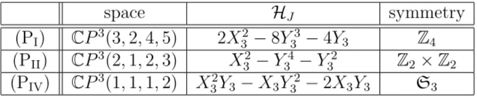
∈ C are parameters. These equations are investigated by means of the weighted projective spaces C P

(p, q, r, s) with natural numbers p, q, r, s given by

(P

) (p, q, r, s) = (3, 2, 4, 5), (P

) (p, q, r, s) = (2, 1, 2, 3), (P

) (p, q, r, s) = (1, 1, 1, 2).

These numbers will be determined by the Newton diagrams of the equations or the versal deformations of a certain class of dynamical systems. The weighted projective space C P

(p, q, r, s) is a three dimensional compact orbifold (toric variety) with singularities, see Sec.2 for the definition.

(P

), (P

) and (P

) are given as differential equations on C P

(p, q, r, s), which is regarded as a compactification of the original phase space C

of the Painlev´ e equations. The Painlev´ e equations are invariant under the Z

action of the form

(x, y, z) 7→ (ω

x, ω

y, ω

z), ω := e

, (1.4) with p, q, r, s as above. As a result, it turns out that (P

), (P

) and (P

) are well defined as meromorphic differential equations on C P

(p, q, r, s).

The space C P

(p, q, r, s) is decomposed as

C P

(p, q, r, s) = C

/ Z

∪ C P

(p, q, r), (disjoint). (1.5) This means that C P

(p, q, r, s) is a compactification of C

/ Z

obtained by attaching a 2-dim weighted projective space C P

(p, q, r) at infinity. The Painlev´ e equations (P

), (J = I, II, IV) divided by the Z

action are given on C

/ Z

, and the 2-dim space C P

(p, q, r) describes the behavior of (P

) near infinity (i.e. x = ∞ or y = ∞ or z = ∞ ). On the “infinity set” C P

(p, q, r), there exist several singularities of the foliation defined by solutions of the equation. Some of them correspond to movable poles of (P

), and the others correspond to the irregular singular point z = ∞ . Local properties of these singularities of the foliation will be investigated by means of dynamical systems theory. Our main results include

• the fact that the Painlev´ e equations are locally transformed into integrable systems near movable singularities,

• a simple proof of the fact that any solutions of (P

) are meromorphic on C ,

• a simple construction of the symplectic atlas of Okamoto’s space of initial conditions,

• for (P

), a geometric interpretation of the Painlev´ e coordinates defined by { x = uw

− 2w

−

zw −

w

y = w

, (1.6)

which was introduced in his original work [26] to prove the Painlev´ e property of (P

),

• a geometric interpretation of the Boutroux coordinates introduced in [2] to investigate the irregular singular point of (P

) and (P

).

In Sec.2, the Newton diagram of the Painlev´ e equation will be introduced to find a suitable weight of the weighted projective space C P

(p, q, r, s). Furthermore, it is shown that the Painlev´ e equations are obtained from certain problems of dynamical systems theory. Such a relationship between the Painlev´ e equations and dynamical systems proposes normal forms of the Painlev´ e equations because for dynamical systems (germs of vector fields), the normal form theory have been well developed.

In Sec.3, with the aid of the orbifold structure of C P

(p, q, r, s) and the Poincar´ e linearization theorem, it will be shown that (P

), (P

) and (P

) are locally trans- formed into integrable systems near each movable singularities. For example, (P

) and (P

) can be transformed into the equations y

= 6y

and y

= 2y

, respectively.

See Sec.3 for the result for (P

). This fact was first obtained by [10] for (P

), in which the transformed equation y

= 6y

is called the singular normal form. Our proof is based on the Poincar´ e linearization theorem and it is easily applied to other Painlev´ e equations, including (P

), (P

) (P

) and higher order Painlev´ e equations [7]. By using this result, a simple proof of the Painlev´ e property is proposed; that is, a new proof of the fact that any solutions of (P

), (P

) and (P

) are meromorphic on C will be given.

In Sec.4, the weighted blow-up will be introduced to construct the spaces of ini-

tial conditions. For a polynomial system, a manifold E(z) parameterized by z ∈ C

is called the space of initial conditions if any solution gives a global holomorphic sec-

tion on the fiber bundle P = { (x, z) | x ∈ E(z), z ∈ C} over C . It is remarkable that

only one, two and three times blow-ups are sufficient to obtain the spaces of initial

conditions for (P

), (P

) and (P

), respectively, if we use suitable weights, while

Okamoto performed blow-ups (without weights) eight times to obtain the space of

initial conditions [24]. Further, our method easily provides a symplectic atlas of

the space of initial conditions. Then, each Painlev´ e equation is characterized as a

unique Hamiltonian system on the space of initial conditions admitting a holomor-

phic symplectic form. Symplectic atlases of the spaces of initial conditions were first

obtained by Takano et al. [28, 22, 23] only for (P

) to (P

), while left open for

(P

). In the present paper, the orbifold structure plays an important role to obtain

a symplectic atlas for (P

). See also Iwasaki and Okada [19] for the orbifold setting

of (P

).

By the weighted blow-up of C P

(3, 2, 4, 5) for (P

), we will recover the famous Painlev´ e coordinates (1.6) in a purely geometric manner. Painlev´ e found the coordi- nate transformation (1.6) in an analytic way to prove the Painlev´ e property of (P

) (see [15]). From our approach based on the weighted projective space, the Painlev´ e coordinates prove to be nothing but the Darboux coordinates of the nonsingular algebraic surface M (z) defined by

V

= U W

+ 2zW

+ 4W,

which admits a holomorphic symplectic form, where z ∈ C is an independent variable of (P

) and it is a parameter of the surface. Our space of initial conditions is obtained by glueing C

(the original space for dependent variables) and the surface M (z) by a symplectic mapping. Then, (P

) is a Hamiltonian system with respect to the symplectic form. Since (1.6) is a one-to-two transformation, an orbifold setting is essential to give a geometric meaning to the Painlev´ e coordinates; the orbifold C P

(3, 2, 4, 5) provides a natural Z

-action which makes (1.6) a one-to-one transformation.

In Sec.5, the characteristic indices for (P

), (P

) and (P

) will be defined. A few simple properties such as a relation with the Kovalevskaya exponents and the weights of C P

(p, q, r, s) will be given.

In Sec.6, the Boutroux coordinates will be introduced. It is shown that the weighted blow-ups of C P

(p, q, r, s) constructed in Sec.4 also includes the space of initial conditions written in the Boutroux coordinates. Further, we will show that autonomous Hamiltonian systems are embedded in the Boutroux coordinates.

In Sec.7, the extended affine Weyl group for (P

) and (P

) will be considered.

The action of the group on the original chart C

is extended to a birational transformation on C P

(p, q, r, s). It is proved that on the “infinity set”, C P

(p, q, r), the foliation defined by an autonomous Hamiltonian system is invariant under the automorphism group Aut(X), where X = A

for (P

) and X = A

for (P

).

In Sec.8, a cellular decomposition of the weighted blow-ups of C P

(p, q, r, s) will be given. We will show that the weighted blow-ups of C P

(p, q, r, s) is naturally decomposed into the fiber space for (P

) (a fiber bundle over C whose fiber is the space of initial conditions), a certain elliptic fibration over the moduli space of complex tori, and the projective curve C P

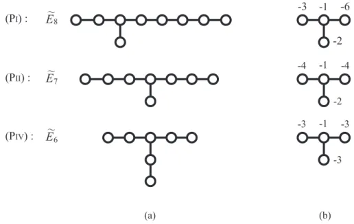
. We also show that the extended Dynkin diagrams of type ˜ E

, E ˜

and ˜ E

are hidden in the weighted blow-ups of C P

(p, q, r, s).

An approach using toric varieties is also applicable to the third, fifth, sixth

Painlev´ e equations and higher order Painlev´ e equations [7, 8]. The Hamiltonian

functions of the third, fifth, sixth Painlev´ e equations are not polynomial in z, and

the Newton diagrams of them are degenerate; weights of them include nonpositive

integers. Hence, the study of the third, fifth, sixth Painlev´ e equations using toric

varieties will be reported in a separated paper [8].

2 Weighted projective spaces

In this section, a weighted projective space C P

(p, q, r, s) is defined and the first, sec- ond and fourth Painlev´ e equations are given as meromorphic equations on C P

(p, q, r, s) for suitable integers p, q, r, s. Such integers p, q, r, s will be found via the Newton di- agrams of the equations. We also give a relationship between the Painlev´ e equations and the normal form theory of dynamical systems, which proposes normal forms of the Painlev´ e equations.

2.1 Newton diagram

Let us consider the system of polynomial differential equations dx

dz = f

(x, y, z), dy

dz = f

(x, y, z). (2.1)

The exponent of a monomial x

y

z

included in f

is defined by (i − 1, j, k + 1), and by (i, j − 1, k + 1) for one in f

. Each exponent specifies a point of the integer lattice in R

. The Newton polyhedron of the system (2.1) is the convex hull of the union of the positive quadrants R

with vertices at the exponents of the monomials which appear in the system. The Newton diagram of the system is the union of the compact faces of its Newton polyhedron. Suppose that the Newton diagram consists of only one compact face. Then, there is a tuple of positive integers (p

, p

, r, s) such that the compact face lies on the plane p

x + p

y + rz = s in R

. In this case, the function f

(i = 1, 2) satisfies

f

(λ

x, λ

y, λ

z) = λ

f

(x, y, z), for any λ ∈ C .

We also consider the perturbation of the system (2.1) of the form dx

dz = f

(x, y, z) + g

(x, y, z), dy

dz = f

(x, y, z) + g

(x, y, z). (2.2) Suppose that g

(λ

x, λ

y, λ

z) ∼ o(λ

) for i = 1, 2 as λ → ∞ . This implies that exponents of any monomials included in g

lie on the lower side of the plane p

x + p

y + rz = s.

The Newton polyhedron of the first Painlev´ e equation (1.1) is defined by three points ( − 1, 2, 1), ( − 1, 0, 2) and (1, − 1, 1). Hence, the Newton diagram consists of the unique face which lies on the plane 3x + 2y + 4z = 5. One of the normal vector to the plane is given by e

= ( − 3/5, − 2/5, − 4/5). Put e

= (1, 0, 0), e

= (0, 1, 0) and e

= (0, 0, 1). Then, the toric variety defined by the fan made up of the cones generated by all proper subsets of { e

, e

, e

, e

} is the weighted projective space C P

(3, 2, 4, 5) [11].

Next, let us consider the second Painlev´ e equation (1.2) with f = (2y

+ yz, x)

and g = (α, 0). The Newton polyhedron of f = (f

, f

) is defined by three points

( − 1, 3, 1), ( − 1, 1, 2), (1, − 1, 1), and the Newton diagram is given by the unique face on the plane 2x + y + 2z = 3. The associated toric variety is C P

(2, 1, 2, 3).

For the fourth Painlev´ e equation (1.3), put f = ( − x

+2xy+2xz, − y

+2xy − 2yz) and g = ( − 2θ

, − 2κ

). The Newton diagram of f = (f

, f

) is given by the unique face on the plane x + y + z = 2 passing through the exponents (1, 0, 1), (0, 1, 1) and (0, 0, 2). The associated toric variety is C P

(1, 1, 1, 2).

In what follows, the weights (p, q, r, s) denote (3, 2, 4, 5), (2, 1, 2, 3) and (1, 1, 1, 2), respectively, for (P

), (P

) and (P

).

The weighted degree of a monomial x

y

z

with respect to the weight (p, q, r) is defined by deg(x

y

z

) = pi + qj + rk. The weighted degree of a polynomial f = ∑

a

x

y

z

is defined by deg(f ) = max

i,j,k

{ deg(x

y

z

) | a

̸ = 0 } .

For (P

), (P

) and (P

) with the weights (p, q, r) = (3, 2, 4), (2, 1, 2) and (1, 1, 1), respectively, the weighted degrees of the Hamiltonian functions are

deg(H

) = 6, deg(H

) = 4, deg(H

) = 3.

They satisfy deg(H

) = s + 1 (J = I, II, IV). Further, it will be shown that they coincide with the Kovalevskaya exponents (Sec.2.3) and the characteristic index λ

(Sec.5).

2.2 Weighted projective space

Let U e be a complex manifold and Γ a finite group acting analytically and effectively on U. In general, the quotient space e U /Γ is not a smooth manifold if the action e has fixed points. Roughly speaking, a (complex) orbifold M is defined by glueing a family of such spaces U e

/Γ

; a Hausdorff space M is called an orbifold if there exist an open covering { U

} of M and homeomorphisms φ

: U

≃ U e

/Γ

. See [29] for more details. In this article, only quotient spaces of the form C

/ Z

will be used.

Consider the weighted C

-action on C

defined by

(x, y, z, ε) 7→ (λ

x, λ

y, λ

z, λ

ε), λ ∈ C

:= C\{ 0 } , (2.3) where the weights p, q, r, s are positive integers. We assume 1 ≤ p, q, r ≤ s without loss of generality. Further, we suppose that any three numbers among them have no common divisors. The quotient space

C P

(p, q, r, s) := C

\{ 0 } / C

gives a three dimensional orbifold called the weighted projective space. The inhomo- geneous coordinates of C P

(p, q, r, s), which give an orbifold structure of C P

(p, q, r, s), are defined as follows.

The space C P

(p, q, r, s) is defined by the equivalence relation on C

\{ 0 }

(x, y, z, ε) ∼ (λ

x, λ

y, λ

z, λ

ε).

(i) When x ̸ = 0,

(x, y, z, ε) ∼ (1, x

y, x

z, x

ε) =: (1, Y

, Z

, ε

).

Due to the choice of the branch of x

, we also obtain

(Y

, Z

, ε

) ∼ (e

Y

, e

Z

, e

ε

),

by putting x 7→ e

x. This implies that the subset of C P

(p, q, r, s) such that x ̸ = 0 is homeomorphic to C

/ Z

, where the Z

-action is defined as above.

(ii) When y ̸ = 0,

(x, y, z, ε) ∼ (y

x, 1, y

z, y

ε) =: (X

, 1, Z

, ε

).

Because of the choice of the branch of y

, we obtain

(X

, Z

, ε

) ∼ (e

X

, e

Z

, e

ε

).

Hence, the subset of C P

(p, q, r, s) with y ̸ = 0 is homeomorphic to C

/ Z

. (iii) When z ̸ = 0,

(x, y, z, ε) ∼ (z

x, z

y, 1, z

ε) =: (X

, Y

, 1, ε

).

Similarly, the subset { z ̸ = 0 } ⊂ C P

(p, q, r, s) is homeomorphic to C

/ Z

. (iv) When ε ̸ = 0,

(x, y, z, ε) ∼ (ε

x, ε

y, ε

z, 1) =: (X

, Y

, Z

, 1).

The subset { ε ̸ = 0 } ⊂ C P

(p, q, r, s) is homeomorphic to C

/ Z

. This proves that the orbifold structure of C P

(p, q, r, s) is given by

C P

(p, q, r, s) = C

/ Z

∪ C

/ Z

∪ C

/ Z

∪ C

/ Z

.

The local charts (Y

, Z

, ε

), (X

, Z

, ε

), (X

, Y

, ε

) and (X

, Y

, Z

) defined above are called inhomogeneous coordinates as the usual projective space. Note that they give coordinates on the lift C

, not on the quotient C

/ Z

(i = p, q, r, s). Therefore, any equations written in these inhomogeneous coordinates should be invariant under the corresponding Z

actions.

In what follows, we use the notation (x, y, z) for the fourth local chart instead of (X

, Y

, Z

) because the Painlev´ e equation will be given on this chart.

The transformations between inhomogeneous coordinates are give by

 



 

x = ε

= X

ε

= X

ε

y = Y

ε

= ε

= Y

ε

z = Z

ε

= Z

ε

= ε

.

(2.4)

We give the differential equation defined on the (x, y, z)-coordinates as dx

dz = f(x, y, z), dy

dz = g(x, y, z), (2.5)

where f and g are rational functions. By the transformation (2.4), the above equa- tion is rewritten as equations on the other inhomogeneous coordinates (Y

, Z

, ε

), (X

, Z

, ε

) and (X

, Y

, ε

). It is easy to verify that the equations written in the other inhomogeneous coordinates are rational if and only if Eq.(2.5) is invariant under the Z

-action

(x, y, z) 7→ (ω

x, ω

y, ω

z), ω = e

. (2.6) In this case, the equations written in (Y

, Z

, ε

), (X

, Z

, ε

) and (X

, Y

, ε

) are invariant under the Z

, Z

and Z

-actions, respectively. Hence, a tuple of these four equations gives a well-defined rational differential equation on C P

(p, q, r, s).

When x = ∞ or y = ∞ or z = ∞ , we have ε

= 0 or ε

= 0 or ε

= 0. In this case, the transformation (2.4) results in

{

Y

= X

= Y

X

,

Z

= Z

X

= X

. (2.7) The space obtained by glueing three copies of C

by the above relations gives the 2-dim weighted projective space C P

(p, q, r). Thus, we have obtained the decom- position

C P

(p, q, r, s) = C

/ Z

∪ C P

(p, q, r), (disjoint). (2.8) On the covering space C

of C

/ Z

, the coordinates (x, y, z) is assigned and Eq.(2.5) is given. The equation on C P

(p, q, r) is obtained by putting ε

= 0 or ε

= 0 or ε

= 0, which describes the behavior of Eq.(2.5) near infinity;

C P

(p, q, r) = { ε

= 0 } ∪ { ε

= 0 } ∪ { ε

= 0 } . (2.9) Now we give the first Painlev´ e equation (1.1) on the fourth local chart of C P

(3, 2, 4, 5).

By (2.5), (P

) is transformed into the following equations dY

dε

= 3 − 12Y

− 2Y

Z

ε

( − 30Y

− 5Z

) , dZ

dε

= 3ε

− 24Y

Z

− 4Z

ε

( − 30Y

− 5Z

) , (2.10) dX

dε

= − 12 − 2Z

+ 3X

5X

ε

, dZ

dε

= − 2ε

+ 4X

Z

5X

ε

, (2.11)

dX

dε

= 24Y

+ 4 − 3X

ε

− 5ε

, dY

dε

= 4X

− 2Y

ε

− 5ε

, (2.12)

on the other inhomogeneous coordinates. Although the transformations (2.4) have branches, the above equations are rational due to the symmetry (2.6) of (P

). Hence, they define a rational ODE on C P

(3, 2, 4, 5) in the sense of an orbifold.

Next, we give the second Painlev´ e equation (1.2) on the fourth local chart of

C P

(2, 1, 2, 3). By (2.4), (P

) is transformed into the following equations dY

dε

= − 2 + Y

(2Y

+ Y

Z

+ αε

) 3ε

(2Y

+ Y

Z

+ αε

) , dZ

dε

= − 2ε

+ 2Z

(2Y

+ Y

Z

+ αε

)

3ε

(2Y

+ Y

Z

+ αε

) , (2.13) dX

dε

= 2X

− (2 + Z

+ αε

)

3X

ε

, dZ

dε

= 2X

Z

− ε

3X

ε

, (2.14)

dX

dε

= 4Y

+ 2Y

+ 2αε

− 2X

ε

− 3ε

, dY

dε

= 2X

− Y

ε

− 3ε

, (2.15)

on the other local charts. They define a rational ODE on C P

(2, 1, 2, 3) because of the symmetry (2.6) of (P

).

Similarly, we give the fourth Painlev´ e equation (1.3) on the fourth local chart of C P

(1, 1, 1, 2). The equations written in the other inhomogeneous coordinates are given by

 

 

 

 dY

dε

= − Y

+ 2Y

− 2Y

Z

− 2κ

ε

+ Y

(1 − 2Y

− 2Z

+ 2θ

ε

) 2ε

(1 − 2Y

− 2Z

+ 2θ

ε

) , dZ

dε

= ε

+ Z

(1 − 2Y

− 2Z

+ 2θ

ε

) 2ε

(1 − 2Y

− 2Z

+ 2θ

ε

) ,

(2.16)

 

 

 

 dX

dε

= − X

+ 2X

+ 2X

Z

− 2θ

ε

+ X

(1 − 2X

+ 2Z

+ 2κ

ε

) 2ε

(1 − 2X

+ 2Z

+ 2κ

ε

) , dZ

dε

= ε

+ Z

(1 − 2X

+ 2Z

+ 2κ

ε

) 2ε

(1 − 2X

+ 2Z

+ 2κ

ε

) ,

(2.17)

 

 

 

 dX

dε

= − X

+ 2X

Y

+ 2X

− 2θ

ε

− X

ε

− 2ε

, dY

dε

= − Y

+ 2X

Y

− 2Y

− 2κ

ε

− Y

ε

− 2ε

.

(2.18)

They define a rational ODE on C P

(1, 1, 1, 2).

2.3 Laurent series of solutions

Let us derive the Laurent series of solutions of the Painlev´ e equations and define the Kovalevskaya exponent. Since any solutions of (P

), (P

) and (P

) are mero- morphic, a general solution admits the Laurent series with respect to T := z − z

, where z

is a movable pole.

For the first Painlev´ e equation (P

), the Laurent series of a general solution is given by

( x y

)

= ( − 2

0 )

T

+ ( 0

1 )

T

− ( z

/5

0 )

T −

( 1/2 z

/10

) T

+

( A

− 1/6 )

T

+ · · · ,

(2.19)

where A

is an arbitrary constant.

For the second Painlev´ e equation (P

), the Laurent series are expressed in two ways as

(i) ( x

y )

= ( 1

0 )

T

− ( 0

1 )

T

+ ( z

/6

0 )

+

( (1 − α)/2 z

/6

) T +

( A

B

)

T

+ · · · , (ii)

( x y

)

= − ( 1

0 )

T

+ ( 0

1 )

T

− ( z

/6

0 )

−

( (1+α)/2 z

/6

) T −

( A

B

)

T

+ · · · , where B

= (1 − α)/4 for the first line, B

= (1 + α)/4 for the second line and A

is an arbitrary constant.

For the fourth Painlev´ e equation (P

), there are three types of the Laurent series given by

(i) ( x

y )

= ( 1

0 )

T

+ ( z

0 )

+

( (2 + z

− 2θ

+ 4κ

)/3 2κ

) T +

( A

B

)

T

+ · · · , (ii)

( x y

)

= ( − 1

− 1 )

T

+ ( z

− z

)

+ 1 3

( 6 − z

+ 2θ

− 4κ

− 6 − z

− 4θ

+ 2κ

)

T + ( A

B

)

T

+ · · · , (iii)

( x y

)

= ( 0

1 )

T

− ( 0

z

)

−

( 2θ

(2 − z

− 4θ

+ 2κ

)/3 )

T + ( A

B

)

T

+ · · · . A

is an arbitrary constant and B

is a certain constant depending on A

.

Let us consider a general system (2.2) satisfying the assumptions given in Sec.2.1;

the Newton diagram consists of one compact face that lies on the plane p

x + p

y + rz = s, and g

satisfies g

(λ

x, λ

y, λ

z) ∼ o(λ

). In this case, the system has a formal series solution of the form

 

 



 

 

x(z) =

∑

A

(z − z

)

, y(z) =

∑

B

(z − z

)

.

(2.20)

The coefficients A

and B

are determined by substituting the series into the equa- tion. If the series solution represents a general solution, it includes an arbitrary parameter other than z

. The Kovalevskaya exponent κ is defined to be the least integer n such that the coefficient (A

, B

) includes an arbitrary parameter. For the Laurent series solution of (P

), κ = 6. For (P

), κ = 4 for both series, and for (P

), κ = 3 for all Laurent series solutions. Note that the Kovalevskaya exponents of them coincide with the weighted degrees of Hamiltonian functions given in Sec.2.1.

In Sec.5, it is shown that the Kovalevskaya exponent coincides with an eigenvalue

of a Jacobi matrix of a certain vector field, and the exponent is invariant under the

actions of automorphisms of C P

(p, q, r, s). See [1, 3, 7, 18, 31, 32] for more general

definition and properties of the Kovalevskaya exponent.

2.4 Relation with dynamical systems theory

In this section, a relationship between the Painlev´ e equations and the normal form theory of dynamical systems is shown. The Painlev´ e equations will be obtained from certain singular perturbed problems of vector fields.

Let us consider a singular perturbation problem of the form { x ˙ = f (x, z, ε),

˙

z = εg(x, z, ε), (2.21)

where x ∈ R

, z ∈ R

, and (f , g) is a smooth vector field on R

parameterized by a small parameter ε ∈ R . The dot ( ˙ ) denotes the derivative with respect to time t ∈ R . Such a system is called a fast-slow system because it is characterized by two different time scales; fast motion x and slow motion z. This structure yields nonlinear phenomena such as a relaxation oscillation, which is observed in many physical, chemical and biological problems. See Grasman [14], Hoppensteadt and Izhikevich [17] and references therein for applications of fast-slow systems. The unperturbed system is defined by putting ε = 0 as

x ˙ = f (x, z, 0), z ˙ = 0. (2.22) Since z is a constant for the unperturbed system, it is regarded as a parameter of the fast system ˙ x = f (x, z, 0).

It is known that when f ∼ O(1) as ε → 0 in some region of R

, the dynamics of (2.21) is approximately governed by the first system ˙ x = f (x, z, 0), and when f ∼ 0 while Df ∼ O(1), the dynamics of (2.21) is approximately governed by the slow system ˙ z = εg(φ(z), z, 0), where Df is the derivative of f with respect to x and φ is a function satisfying f (φ(z), z, 0) = 0. However, if both of f and Df are nearly equal to zero, both of the fast and slow motion should be taken into account and a nontrivial dynamics may occur. The condition

f (x

, z

, 0) = 0, Df (x

, z

, 0) = 0

implies that the first system ˙ x = f (x, z, 0) undergoes a bifurcation at x = x

with a bifurcation parameter z = z

. A type of a bifurcation almost determines the local dynamics of (2.21) around (x, z) = (x

, z

)

For the most generic case, in which the fast system undergoes a saddle-node bifurcation, it is well known that a local behavior of (2.21) is governed by the Airy equation d

u/dz

= zu. In particular, the asymptotic analysis of the Airy function plays an important role, see [20, 13]. Chiba [5] found that when the fast system

˙

x = f (x, z, 0) undergoes a Bogdanov-Takens bifurcation, then a local behavior of

(2.21) is determined by the asymptotic analysis of Boutroux’s tritronqu´ ee solution

of the first Painlev´ e equation. This result was applied to prove the existence of a

periodic orbit and chaos in a certain biological system [6]. Here, we will demonstrate

how the first, second and fourth Painlev´ e equations are obtained from fast-slow

systems. For a normal form and versal deformation of germs of vector fields, the

readers can refer to [9].

Suppose that a one-dimensional dynamical system ˙ x = f(x) lies on a codimension 1 bifurcation at x = 0. This means that f satisfies

f (0) = f

(0) = 0, f

(0) ̸ = 0. (2.23) The normal form is given by f (x) = x

, and its versal deformation is ˙ x = x

+ z or

˙

x = x

+zx with a deformation parameter z ∈ R . The former is called a saddle-node bifurcation and the latter is a transcritical bifurcation. The fast-slow system having the saddle-node as an unperturbed fast system is written by

˙

x = x

+ z + εf (x, z, ε), z ˙ = εg(x, z, ε). (2.24) We also assume the generic condition g(0, 0, 0) ̸ = 0 so that we can write g(x, z, ε) = 1 + O(x, z, ε) without loss of generality. In order to investigate the local behavior of the system near (x, z) = (0, 0) for a small ε, we rewrite Eq.(2.24) as a three dimensional system 





˙

x = x

+ z + εf(x, z, ε)

˙

z = ε + ε · O(x, z, ε)

˙ ε = 0,

(2.25) by adding the trivial equation ˙ ε = 0. For this system, we perform the weighted blow-up at the origin defined by



 x z ε



 =



 r

r

Z

r

ε



 =



 r

X

r

r

ε



 =



 r

X

r

Z

r



 . (2.26)

The weight (exponents of r

’s) (1, 2, 3) can be found by the Newton diagram of Eq.(2.25) as in Sec.2.1. The exceptional divisor of the blow-up is C P

(1, 2, 3) given by the set { r

= 0 } ∪ { r

= 0 } ∪ { r

= 0 } . On the (X

, Z

, ε

) chart, Eq.(2.25) is written as

X ˙

= r

X

+ r

Z

+ O(r

), Z ˙

= r

+ O(r

), r ˙

= 0. (2.27) This is equivalent to

dX

dZ

= X

+ Z

+ O(r

) 1 + O(r

) .

In particular, on the exceptional divisor C P

(1, 2, 3), it is reduced to the Riccati equation

dX

dZ

= X

+ Z

, (2.28)

which is equivalent to the Airy equation u

= − Z

u by X

= − u

/u. Similarly, if we

use the transcritical bifurcation as the fast system and apply the weighted blow-up

with the weight (1, 1, 2), we obtain the Hermite equation u

− Z

u

− αu = 0 on

the exceptional divisor. See [4] for the analysis of the Airy equation based on the geometry of C P

(1, 2, 3).

The Painlev´ e equations are obtained from codimension 2 bifurcations in a similar manner. Suppose that a 2-dim system of (x, y) undergoes a generic codimension 2 bifurcation called the Bogdanov-Takens bifurcation. The normal form is given by

˙

x = y

+ xy, y ˙ = x; that is, the linear part has two zero eigenvalues. Its versal

deformation is {

˙

x = y

+ xy + z,

˙

y = x, (2.29)

where z is a deformation parameter. The fast-slow system having it as an unper- turbed fast system is written by

 

 

 



˙

x = y

+ xy + z + εf

(x, y, z, ε)

˙

y = x + εf

(x, y, z, ε),

˙

z = ε + ε · O(x, y, z, ε),

˙ ε = 0,

(2.30)

where the trivial equation ˙ ε = 0 is added as before. For this system, we introduce the weighted blow-up with the weight (3, 2, 4, 5) defined by



 

 x y z ε



 

 =



 

 r

r

Y

r

Z

r

ε



 

 =



 

 r

X

r

r

Z

r

ε



 

 =



 

 r

X

r

Y

r

r

ε



 

 =



 

 r

X

r

Y

r

Z

r



 

 . (2.31)

The weight (3, 2, 4, 5) can be obtained via the Newton diagram of the system (2.30).

The exceptional divisor of the blow-up is the weighted projective space C P

(3, 2, 4, 5) given as the set { r

= 0 } ∪ { r

= 0 } ∪ { r

= 0 } ∪ { r

= 0 } . Transforming the system (2.30) to the (X

, Y

, Z

, r

) chart, we obtain

 



X ˙

= r

Y

+ r

Z

+ O(r

), Y ˙

= r

X

+ O(r

),

Z ˙

= r

+ O(r

).

As r

→ 0, it is reduced to the first Painlev´ e equation dX

/dZ

= Y

+Z

, dY

/dZ

= X

. This implies that the dynamics on the divisor C P

(3, 2, 4, 5) is governed by the compactified first Painlev´ e equation, and a local behavior of the system (2.30) near (x, y, z) = (0, 0, 0) can be investigated by a global analysis of the first Painlev´ e equation.

Next, we consider a 2-dim system that undergoes a Bogdanov-Takens bifurcation with Z

-symmetry (x, y) 7→ ( − x, − y). The versal deformation of the normal form

is given by {

˙

x = y

− xy

+ zy,

˙

y = x, (2.32)

with a deformation parameter z. The fast-slow system having it as an unperturbed fast system is written by

 

 

 



˙

x = y

− xy

+ zy + εf

(x, y, z, ε)

˙

y = x + εf

(x, y, z, ε),

˙

z = ε + ε · O(x, y, z, ε),

˙ ε = 0.

(2.33)

For this system, we introduce the weighted blow-up with the weight (2, 1, 2, 3), which is found by the Newton diagram of the system (2.33). On the (X

, Y

, Z

, r

) chart, it provides

 



X ˙

= r

Y

+ r

Z

Y

− r

X

Y

+ r

f

(r

X

, r

Y

, r

Z

, r

), Y ˙

= r

X

+ O(r

),

Z ˙

= r

+ O(r

).

Note that r

f

(r

X

, r

Y

, r

Z

, r

) = αr

+ O(r

), where α := f

(0, 0, 0, 0). As r

→ 0, this system is reduced to the second Painlev´ e equation X

= Y

+ Y

Z

+ α, Y

= X

with a parameter α.

Finally, we consider a 2-dim system that undergoes a Bogdanov-Takens bifurca- tion with Z

-symmetry. Using the complex variable η ∈ C , the normal form of such a bifurcation is given by ˙ η = η | η |

+ η

. Note that this system is invariant under the Z

action η 7→ e

η. The versal deformation of the normal form is

˙

η = η | η |

+ η

+ ηz. (2.34)

where z ∈ C is a deformation parameter. Putting η = x + iy, z = z

+ iz

yields { x ˙ = x

− y

+ z

x − z

y + O(η

),

˙

y = − 2xy + z

y + z

x + O(η

).

We assume z

= 0 so that the above system may become a Hamiltonian system, and change the notation z

7→ z to obtain

{ x ˙ = x

− y

− zy + O(η

),

˙

y = − 2xy + zx + O(η

).

The fast-slow system having it as an unperturbed fast system is written by

 

 

 



˙

x = x

− y

− zy + O(η

) + εf

(x, y, z, ε)

˙

y = − 2xy + zx + O(η

) + εf

(x, y, z, ε),

˙

z = ε + ε · O(x, y, z, ε),

˙ ε = 0.

(2.35)

For this system, we introduce the weighted blow-up with the weight (1, 1, 1, 2).

Moving to the (X

, Y

, Z

) chart and putting r

= 0 as before, it turns out that the system (2.35) is reduced the system

 



  dX

dZ

= X

− Y

− Z

Y

+ α

dY

dZ

= − 2X

Y

+ Z

Y

+ α

,

(2.36)

where α

:= f

(0, 0, 0, 0) is a constant (i = 1, 2). This is equivalent to the fourth Painlev´ e equation (1.3) through an affine transformation of (X

, Y

).

Bifurcation type Exceptional divisor Equation on the divisor

saddle-node C P

(1, 2, 3) Airy

transcritical C P

(1, 1, 2) Hermite Bogdanov-Takens (BT) C P

(3, 2, 4, 5) (P

)

BT with Z

symmetry C P

(2, 1, 2, 3) (P

) BT with Z

symmetry C P

(1, 1, 1, 2) (P

)

Table 1: Differential equations obtained by the weighted blow-up of the fast-slow systems.

The results are summarized in Table 1. It is remarkable that the weights (p, q, r, s) derived in Sec.2.1 via the Newton diagrams are determined only by the ver- sal deformations of the codimension 2 bifurcations. Further, the Painlev´ e equations are obtained in a compactified manner on C P

(p, q, r, s), which is the exceptional divisor of the weighted blow-up.

3 Singular normal forms and the Painlev´ e prop- erty

Recall that a singularity z = z

of a solution of a differential equation is called movable if the position of z

depends on the choice of an initial condition. In this section, we give local analysis near such movable singularities based on the normal form theory. Our purpose is to show that near movable singularities, the Painlev´ e equations are locally transformed into integrable systems called the singular normal form. Further, we will give a new proof of the Painlev´ e property; any solutions of (P

), (P

) and (P

) are meromorphic on C (for this purpose, we do not use the Laurent series given in Sec.2.3).

3.1 The first Painlev´ e equation

(P

) is given on the weighted projective space C P

(3, 2, 4, 5) as a tuple of equations (1.1), (2.10), (2.11) and (2.12). Coordinate transformations between inhomogeneous coordinates are given by

 



 

x = ε

= X

ε

= X

ε

y = Y

ε

= ε

= Y

ε

z = Z

ε

= Z

ε

= ε

.

(3.1)

Due to the orbifold structure of C P

(3, 2, 4, 5), local charts (Y

, Z

, ε

), (X

, Z

, ε

) and (X

, Y

, ε

) should be divided by the Z

, Z

and Z

actions

(Y

, Z

, ε

) 7→ (ωY

, ω

Z

, ωε

), ω := e

, (3.2) (X

, Z

, ε

) 7→ ( − X

, Z

, − ε

), (3.3) (X

, Y

, ε

) 7→ (iX

, − Y

, − iε

), (3.4) respectively. Indeed, Eqs.(2.10),(2.11),(2.12) are invariant under these actions. For our purposes, it is convenient to rewrite Eqs.(2.10), (2.11) and (2.12) as 3-dim vector fields (autonomous ODEs) given by

 



Y ˙

= 3 − 12Y

− 2Y

Z

, Z ˙

= 3ε

− 24Y

Z

− 4Z

,

˙

ε

= ε

( − 30Y

− 5Z

),

(3.5)

 



X ˙

= ( − 12 − 2Z

+ 3X

)/X

, Z ˙

= ( − 2ε

+ 4X

Z

)/X

,

˙

ε

= 5ε

,

(3.6)

 



X ˙

= 24Y

+ 4 − 3X

ε

, Y ˙

= 4X

− 2Y

ε

,

˙

ε

= − 5ε

,

(3.7) where (˙) = d/dt and t is an additional parameter.

Recall the decomposition (2.8) with (2.9). According to Eqs.(3.5),(3.6),(3.7), the set C P

(3, 2, 4) is an invariant manifold of the vector fields; that is, ε

(t) ≡ 0 when ε

(0) = 0 at an initial time. The dynamics on the invariant manifold describes the behavior of (P

) near infinity. In particular, fixed points of the vector fields play an important role. Vector fields (3.5),(3.6),(3.7) have exactly two fixed points on C P

(3, 2, 4);

(i). (X

, Z

, ε

) = ( ± 2, 0, 0).

Due to the Z

action on the (X

, Z

, ε

)-coordinates, two points (2, 0, 0) and ( − 2, 0, 0) represent the same point on C P

(3, 2, 4, 5) and it is sufficient to consider one of them. We will show that this fixed point corresponds to movable singularities of (P

). By applying the normal form theory of vector fields to this point, we will construct the singular normal form of (P

). In Sec.4, the space of initial conditions for (P

) is constructed by applying the weighted blow-up at this point.

(ii). (X

, Y

, ε

) = (0, ± ( − 6)

, 0)

Again, two points should be identified due to the Z

action on (X

, Y

, ε

). This fixed point corresponds to the irregular singular point of (P

) because ε

= 0 provides z = ∞ .

Note that fixed points obtained from the (Y

, Z

, ε

)-coordinates are the same as

one of the above. For example, the fixed point (Y

, Z

, ε

) = ((1/4)

, 0, 0) is the

same as (X

, Z

, ε

) = ( ± 2, 0, 0) due to (3.1).