Does Product Market Competition Promote
Economic Growth? ―Two Bargaining Systems and Creative Destruction―
著者 MURO Kazunobu
journal or
publication title
明治学院大学経済研究 = The papers and proceedings of economics
volume 153
page range 9‑33
year 2017‑01‑31
URL http://hdl.handle.net/10723/2974
Abstract
Is more intense product market competition good or bad for economic growth? This paper constructs an endogenous growth model with bargaining, and derives an inversed-U-shaped relationship between competition and growth. We compare two bargaining systems of effcient bargaining (EB) and right-to-manage (RTM) in the model of creative destruction. An increase in the bargaining power of labor which decreases the number of researchers always decays growth. If the unemployment rate is high, or if the degree of competition is low, policies for promoting competition are good for growth. Greater competition reduces monopoly rents that induce firms to innovate while it decreases the natural rate of unemployment and increases total employment. Since the degree of competition for maximizing the rate of economic growth in the RTM is larger than in the EB, the optimal competitive strategy for growth depends on which of bargaining systems an economy adopts. When unemployment benefits are low, the positive effect of competition on growth emerges easily because Okun’s law works effectively. We propose strategies for growth.
Keywords: product market competition; strategy for growth; Okun’s law; effcient bargaining (EB); right-to-manage (RTM); employment-creating effect; incentive effect;
unemployment benefit JEL classifications: O31, E24, L16,
1 Introduction
Whether more intense product market competition raises the rate of economic growth is a crucial question. Theoretically, in the innovation-based endogenous growth models1with R&D sector, more intense competition, which reduces markups and monopoly rents that induce firms to innovate, always reduces long-run growth. However, this theoretical result appears to be counterintuitive because monopoly is thought to be the key source of ineffciency. Many economists have believed
『経済研究』(明治学院大学)第 153 号 2017 年
Does Product Market Competition Promote Economic Growth?
―Two Bargaining Systems and Creative Destruction―
*†Kazunobu Muro
दthat competition exerts downward pressure on costs, provides incentives for effcient organization, reduces slack, and drives innovation. Empirical works such as Nickell (1996) [33] and Blundell et al.
(1999) [11] show a positive correlation between competition and productivity growth within a firm or industry, measuring competition either by the number of competitors in the same industry or by the inverse of a market share of profitability index2. Porter (1990) insists that competition forces firms to innovate to survive, and competition is good for growth. Adam Smith commented that “monopoly ... is a great enemy to good management” and insisted on gradual deregulation. Peretto-(2015)-[38]
analyzes transformation from a state of affairs with no profit-driven innovation (Smithian phase) to one with it (Schumpeterian phase). The effect of competition on the growth rate varies with phase.
The purpose of this paper is to derive an inversed-U-shaped relationship between competition and growth, and to propose strategies for growth. In a modern economy within Schumpeterian phase, how does the positive effect of competition on the growth rate appear? There are few theoretical papers to explain the positive effect of competition on growth. There are four approaches at present. First, the R&D with a step-by step. Second, decomposing into research and development.
Third, agency considerations. Fourth, labor market imperfections, which is the one we emphasize in this paper. First, Schumpeterian endogenous growth model of Aghion and Howitt (1992) puts the leapfrogging assumption that the innovator is overtaken by outside researchers, and the model shows a negative effect of competition on innovation. In contrast, the assumption is replaced with a less radical step-by step assumption3in the models of Aghion, Harris, and Vickers (1997) [4], Aghion et al.
(2001) [6], and Aghion et al. (2002) [7]. According to them, there is an inversed-U-shaped relationship between growth and competition. How innovation or productivity growth (the flow of new patent) varies with the degree of competition (measured inversely by the ratio of firm rents to value added or to the asset value of the firm)? They show that when competition is initially low, an increase in competition should result in a faster average innovation rate since the “escape-competition” effects dominates. In contrast, when competition is high, an increase in competition should result in a slower average innovation rate since the “Schumpeterian effects” dominates. Second, Aghion and Howitt (1996) [3] decompose R&D activities into research and development. More competition between new and old product lines induces developers to switch from old to new lines rapidly, inducing a higher level of research and growth. Third, Aghion, Dewatripont, and Rey (1999) [5] analyze incentive effects of competition on technological adoption by non-profit maximizing managers. They shows that with conservative firms whose sole desire is to delay adoption of new technologies, competition tends to increase growth while subsidizing innovation tends to deteriorate it.
Fourth, we try to explain the inversed-U-shaped relationship between growth and competition by focusing on labor market imperfections. Solow (2000) [43] (p 185) insists on an integration of Okun’s law [Okun (1962) [36]] and growth models. Empirically, Daveri and Tabellini
(2000) [15] report a significant negative relationship between growth and unemployment4. Let us still put the leapfrogging assumption adopted by Aghion and Howitt (1992). We consider two bargaining systems. The first is an effcient bargaining (EB) which determines the wage rate as well as employment, proposed by McDonald and Solow (1981) [30]. The second is the bargaining system of the right-to-manage (RTM) which determines only the wage rate by negotiations, and the firm decides employment on the demand schedule for labor. We compare two bargaining systems in the endogenous growth model. There are two opposite effects of promoting competition. The positive effect of competition on employment is what we call the “employment-creating effect”. On the other hand, the negative effect of competition on the monopolistic profit and the incentive to the R&D is what we call the “incentive effect”5. When labor has some bargaining power, policies for promoting competition increase total employment. This is because more intense competition increases unemployment benefits and decreases the rate of unemployment. If the employment-creating effect dominates the incentive effect, competition fosters growth.
We show that when the unemployment rate is high to begin with, more intense competition, which decreases the unemployment rate, increases the rate of economic growth. This is because the employment-creating effect dominates. On the other hand, when the unemployment rate is low, a decrease in the degree of competition, which increases the unemployment rate, increases the rate of economic growth. This is because the incentive effect dominates. Therefore, there exists the desired degree of competition for attaining a maximum rate of economic growth. In an economy where markups in the goods markets are too high, it is desired to reduce markups and natural rate of unemployment for growth. Although the higher markup gives the incentive to R&D, it generates ineffciency, that is to say, a dead weight loss due to monopoly and unemployment. Therefore, there is a trade-off as for promoting competition between the employment-creating effect and the incentive effect.
According to Blanchard and Giavazzi (2003) [10], the unemployment benefit which expresses the reservation wage depends negatively on the rate of unemployment. More intense competition increases the unemployment benefit, which decreases the unemployment rate. Since promoting competition increases total employment, it brings about economic growth through Okun’s law.
Bargaining power of labor does not affect the unemployment benefit and the natural rate of unemployment under the effcient bargaining (EB). On the other hand, under the right-to- manage (RTM), the increase in bargaining power of labor decreases the unemployment benefit and increases the natural rate of unemployment. A decrease in the bargaining power of labor enhances economic growth under two systems.
Empirically, Carmeci and Mauro (2003) [14] and Brauninger and Pannenberg (2002) [13]
emphasize the negative effect of unionization of labor on growth6. Through wage bargaining, the union can capture some of monopoly profits. Since the firm anticipates hold-up, it has less incentive
to invest in R&D. Theoretically, Palokangas (1996) [37], Lingens (2003) [28], and Lingens (2007) [29]
focus on the effect of labor market imperfection on growth. They distinguish low-skilled and high- skilled labor and the union bargains over the low-skilled labor wage. However, they does not focus on the effect of competition on growth. Moreover, in their models, only the wage rate is determined by bargaining, while employments are determined by profit maximization. That is, their bargaining system is only the right-to-manage (RTM). In contrast, we compare the EB and the RTM.
Too much generous unemployment benefit is one of problems in continental European economy. When unemployment benefits are low, it is easy for Okun’s law to hold. Then, we obtain the positive effect of competition on growth. The lower the unemployment benefits is, the employment- creating effects function powerfully.
We propose policy prescriptions. Strategies for growth take three steps. First, the decrease in the bargaining power of labor is good for growth. Furthermore, the lower unemployment benefits are good for growth. Second, we emphasize that the optimal strategy for growth depends on which of bargaining systems an economy adopts because the degree of competition for maximizing the rate of growth in the RTM is larger than in the EB. Given the degree of competition, the switch to more desired bargaining system from EB (RTM) to RTM (EB) is good for growth7. Finally, with goal of maximal rate of growth, adjusting the degree of competition is good for growth. If the natural rate of unemployment is high, the policy promoting competition is good for growth. This paper may be a clue to solve the problem of productivity slowdown and high rate of unemployment suffered in continental Europe.
Shortening patent length implies a kind of policies promoting competition. Finite patent length in the growth model is analyzed by Judd (1985) [25], Iwaisako and Futagami (2003) [21], and Futagami and Iwaisako (2007) [17]. In their models, extending the patent length (that is, strengthening monopoly power) enhances economic growth by raising the rate of return of R&D. In other word, infinite patent length8is good for growth. Therefore, there is still a negative effect of competition on growth in their models.
The remaining paper is organized as follows. Section 2 presents the quality-ladder endogenous growth model with effcient bargaining (EB). Section 3 presents the model with the right-to-manage (RTM). Section 4 compares the two bargaining systems. Section 5 proposes strategies for growth.
Section 6 concludes this paper.
2 The Model with Effcient Bargaining
2.1 Househoolds
We assume that consumers are risk-neural, and they consume all earnings in each instance.
The number of population is denoted by a constant N> 0. The interest rate corresponds to the rate of subjective time preference ρ> 0.
2.2 Final Goods Sector
Final goods are produced according to Yn=Anxαn, where An is the quality of intermediate goods, n is the number of innovations, xn is an input of intermediate goods, and α∈ (0, 1) is a parameter. The production function is constant return to scale in xn and another kind of input whose quality is nor- malized to one. An innovation raises the quality by a factor γ>1, so that innovation process is given by An+1=γAn. The profit-maximization condition of final goods producers is Anαxαn-1=pn, where left- hand side is the marginal product of xn while the right-hand side is the price of intermediate goods pn. 2.3 Intermediate Goods Sector
There is a monopoly firm producing xn. When quality innovation occurs with creation of a new product of qualityAn+1, the intermediate goods xnbecome obsolete and eventually goes out of the market. Then, turn to the product xn+1 available in the market. The patent of the product is protected over infinite horizon. The monopolist sells intermediate goods to final goods sectors, facing a demand curve for the products, that is An αxαn-1=pn. We assume that production of one unit of xn
requires one unit of flow labor services. The profit of the monopolist is given by πn=pnxn-wnxn= Anαxαn-wnxn.
2.4 The R&D Sector
The R&D sector is competitive. When the quality level of intermediate goods is An, the next- generation goods will be invented according to a Poisson distribution with an arrival rate of δ Rn, where δ>0 is R&D productivity or an arrival rate of innovation when one worker is used in research9. Here, Rn is the number of research workers when it is the number of workers used in R&D which aims to generate the (n+1) th innovation. Note that the probability of no innovation is equal to (1-δRn). Denote the sum of the expected present value of future flow of πn+1 by Vn+1. The value of innovation is according to
ρVn+1
=
πn+1+
(δRn+1-
Vn+1)+
(1- -
δRn+1)×
0.
(1)where xn+1 becomes obsolete if xn+1 is invented with a Poisson arrival rate of δRn+1. Here, δRn+1
(-Vn+1)+(1-δRn+1)×0 expresses the expected capital gain. The return from being a successful R&D innovator must be equal to the sum of a profit and capital loss due to an extra innovation.
Since the product becomes obsolete due to an extra innovation, δRn+1 lowers the value of innovation.
As Rn+1 gets higher, Vn+1 falls, which discourages the current R&D and reduces Rn. The innovating firm acquires a monopoly on the production of x that is useful until the next innovation. The n th innovation brings a negative externality (it kills the rents of the firm that produced the n-1 st innovation ) and a positive externality (it makes possible the t+1 st innovation). The labor can work in manufacturing and earn wageswnwhile the labor can engage in R&D and earn Vn+1 with an arrival rate of δ. If there is free entry and risk neutrality in R&D, entry will occur until the cost of conducting R&D is equal to the expected value of the innovation: wnRn+1=δRn+1Vt+1+(1-δRn+1)×0. In equilibrium, we obtain
(2)
2.5 Effcient Bargaining
Let us consider two bargaining systems. First is an effcient bargaining (EB) which determines the wage rate as well as employment. The EB is analyzed in this section. Second is a bargaining of the right-to-manage (RTM) which determines only the wage rate by negotiations, and the firm decides employment unilaterally on the demand schedule for labor. Let us consider the RTM case in the next section.
According to Blanchard and Giavazzi (2003) [10], denote the unemployment benefit (that is the wage equivalent of being unemployed) by f(u)>0, and it is a decreasing function of the unemployment rate u ∈ [0, 1]. That is, we assume f′(u)<0. Higher unemployment makes it more painful to be unemployed. We assume that f(0) is suffciently high and f(1) is suffciently low so that the unemployment rate is strictly between 0 and 1. There does not exist the government, and the unemployment benefits are provided by the employed10.
Labor can get the labor rent which is expressed by the surplus to workers from working in the monopoly firm [wn-Pf(u)]xn, where f(u) can be interpreted as the reservation wage or unemployment benefit, and P is the price of unemployment benefit. Note that the benefit f has some unit. One benefit f corresponds to P intermediate goods. Therefore Pf(u) expresses the nominal unemployment benefit. On the other hand, a monopoly firm gets the profit πn=Anαxαn-wnxn.
The effcient bargaining (EB) chooses not only the wage rate wn but also employment xnto maximize the Nash bargaining product given by
(3)
=
δVn+1.
wn{wmaxn
,
xn}βlog[[wn-
Pf(u)]xn]+
(1-
β)log[Anαxαn-
wnxn],
where β exhibits the bargaining power of labors11.
By differentiating the Nash bargaining with respect to the employment xn, we obtain
(4)
By differentiating the Nash bargaining with respect to the wage rate wn, we obtain
(5)
By substituting (5) into (4), we obtain the monopoly price in terms of unemployment benefit
(6)
where represents the markup and the degree of monopoly in the intermediate goods market.
Here, α=1 corresponds to the perfect competition while α=0 does to the monopoly in the goods market. Note that in the case of effcient bargaining (EB), the markup puts over the unemployment benefit. The optimal wage equation (5) can be written as
(7)
where we use the monopoly price (6). The real wage is set as a weighted average of the reservation wage and the relative price. An increase in β increases the proportion of rents going to workers, and leads to a higher real wage. The monopoly price can be expressed as
(8)
In a basic model of Aghion and Howitt (1992), the monopoly price exhibits the markup over wage rate. On the other hand, in our model with bargaining, the monopoly price is determined by the multiplier 1
(
β+
α(1-
β))
over wage rate. Let us call the multiplier 1(
β+
α(1-
β))
“effective markup”. If bargaining power of labor (β) was null, then the effective markup would correspond to the standard markup which measures the degree of monopoly in the goods market.From (8), we have
=
α(1
-
β) β+
wn
Anαxαn-1 . If xn is constant, A
=
n A
wn wn+1
n+1 holds. We obtain
(9)
The wage rate rises discretely by a factor γ>1.
The monopoly profit under the effcient bargaining (EB) can be computed by
(10)
β
+
αAnαxα-1
n
-
wnπn
=
0.
xn
-
β(1 )
=
[w-
Pf(u)]πn
.
-
β(1 ) xβn
pn
P
=
f(αu),
1αwn
P
=
β pnP
+
f(u)=
f(u) βα
+ ,
)
(
(1-
β)
(1-
β)
=
α(1-
β)<
αpn wn wn
β
+ .
α1
( )
γ
=
wwn+1n
.
πn
=
(-
)=
1-
1 = .
α(1
-
β)wn wn
β
+
α(1-
β)-
β(1 )(1
-
α) β+
pn xn xn wnxn
More intense product market competition decreases the monopoly rents: ∂πn
∂
α <
0. The unionization captures some of monopoly profits because of(11)
2.6 Steady-State Equilibrium in the Effcient Bargaining
From the equation (1), the non-arbitrage condition for the value of innovation is expressed by
(12)
where the right-hand side exhibits income gain. By substituting the profit (10), the wage equalization condition (2), and the wage process (9) into the income gain (12), we can obtain
=
γδ(ρ
+
)
α(1
-
β)-
β(1 )(1
-
α) β+
xn+1n+1
δR . Let us consider the steady-state equilibrium. Dropping the
subscript n, we have(ρ
+
)=
γδ
α(1
-
β)-
β(1 )(1
-
α)β
+
xδR . The equilibrium of labor market is given by R+x=(1-u)N, where the numbers of population (labor force), of unemployed, and of employment are denoted by N, uN, and (1-u)N, respectively. Here, R is the number of researchers in R&D sector while x is the number of manufacturing labor. From the equation (8), not only the wage rate but also the intermediate goods price rise discretely by a factor γ>1. From the equation (6), the relative price
pn
P
=
1 holds at the equilibrium. At the steady state, the natural rate of unemployment is determined according to(13)
where an increase in competition (α) increases the unemployment benefit, reduces the unemployment rate. The wage rate in terms of benefit under the EB is given by wnEB
P
=
β+
α(1-
β). We can compute the steady state equilibrium by(14)
(15)
and (13). By eliminating x from (14) and (15), and by solving for R, we obtain the number of researchers at the steady state in the EB as follows:
∂ β
= -
[ (1
-
α)]2.
wnxn∂πn
<
0 α(1-
β)β
+
=
Vπn+1,n+1
(ρ
+
δRn+1)α
=
f(u),
0<
α<
1,
x= γδ ,
x= N-R,
α(1-β)
-β
(1 )(1-α)
-u
(1 ) β+
ρ+δR
(16)
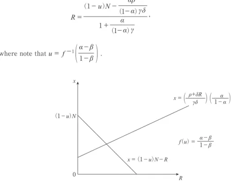
The non-arbitrage condition (14) is an upward-sloping curve while the labor market equilibrium (15) is a downward-sloping curve, in the Figure 1. The condition of a positive numerator in (22) given by (1
-
u)N> (
γδρ)
(
1β- +
(β1)(-
1β-
)αα)
ensures the existence of a steady-state equilibrium.2.7 Expected Rate of Economic Growth
Steady state final output in terms of real time is given by Yt=γntxα. The expected growth rate is computed by
ɡ≡ ∂E
(logY
t)∂t = ∂E
[n
t]∂t
log γ, where∂E[nt]
∂t is the expected number of innovations during a unit time interval. Since innovations follows a Poisson distribution with an arrival rate of δR, the time length between two successive innovations is exponentially distributed and the average time length between one innovation and another is 1
δR, which is the expected time length of one innovation. Therefore, δR is the expected number of innovations for a unit time interval.
Thus, since we have ∂E[nt]
=
δR∂t , the expected growth rate is given by
ɡ
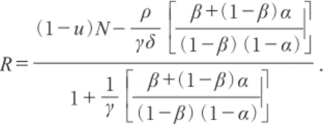
≡δR logγ. If an economic policy increases the number of researchers R, then it is growth-enhancing policy. The expected rate of economic growth is computed by(17)
R
=
ρ γδ 1
+
.
β α
N
-
-
u(1 )
(1
-
β)-
β(1 )(1
-
α)+
β α
(1
-
β)-
β(1 )(1
-
α) 1+
γ
R x
0
(1-u)N
x=(1-u)N-R
(u)=f α
)
x= ρ+δR
(
γδ (1-β)
β+(1-β)(1-α)α
Figure 1: Equilibrium under the Effcient bargaining (EB)
ɡ=δ
(
1-u
1+
)N-
1γ
(
γδ ρ
1β -β +
((1β
1)(-β -β +
(1-α
1)()-β α
1)-α
)α
)
log γ ,
where note that the unemployment rate is given by u=f-1(α).
2.8 Effect of Bargaining Power of Labor on Economic Growth in the EB
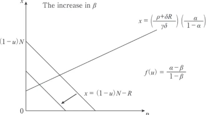
In the EB, the bargaining power of labor (β) does not affect the equation (15). On the other hand, an increase in the bargaining power of labor shifts up the upward-sloping curve (14), and it increases the labor in manufacturing, because of ∂x
∂β
=
12>
0-
β(1 )(1
-
α) . Therefore, we have Proposition 1. See Figure 2.Proposition 1
An increase in the bargaining power of labor decreases the number of researchers but increases the number of manufacturing labor, which decreases the rate of economic growth under the effcient bargaining.
Since an increase in β does not affect the reservation wage, it leaves total employment unchanged. On the other hand, the increase in β increases the real wage and decreases the monopoly profits. The decline of an incentive to innovation forces labor out of the R&D sector. Therefore, it increases labor in manufacturing since the unemployment rate is unchanged.
Empirically, Carmeci and Mauro (2003) [14] and Brauninger and Pannenberg (2002) [13] show the negative effect of unionization of labor on economic growth. Through wage bargaining, the union can capture some of the quasi rents, which are generated by R&D investment of the firm. Since the firm anticipates hold-up, it has less incentive to invest inR &D, compared to a situation without unionization.
0 R
(1-u)N x
x=(1-u)N-R
(u)=f α The increase in β
)
x= ρ+δR
(
γδ (1-β)
β+(1-β)(1-α)α
Figure 2: The increase in the bargaining power of labor in the effcient bargaining (EB)
2.9 Effect of Competition on the Rate of Economic Growth in the EB
The competition12 decreases the rate of unemployment as follows: du
dα
=
1<
0 f u( )´
. More intense competition increases the real wage (7) and decreases the unemployment rate since reservation wage increases. There are two opposite effects of promoting competition. On the one hand, the effect that an increase in competition increases employment is what we call the“employment-creating effect”. On the other hand, the effect that more intense competition decreases monopoly rents and makes the firm have less incentives to R&D investment is what we call the
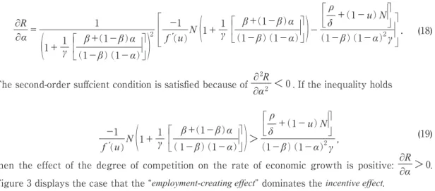
“incentive effect”. The effect of competition on the innovation is given by
∂R
∂α=
1
2
-
1N
-
ρ
δ
+
(1-
u)N γ.
)
(
1+
1γ (
1β- +
(β1)(-
1β-
)αα)
f u( )´
(
1+
1γ (
1β- +
(β1)(-
1β-
)αα)
)
(
1-
β)(1-
α)2 (18)The second-order suffcient condition is satisfied because of ∂2R
∂α2
<
0. If the inequality holds(19)
then the effect of the degree of competition on the rate of economic growth is positive: ∂R
∂α
>
0.Figure 3 displays the case that the “employment-creating effect” dominates the incentive effect.
> ,
ρ
δ
+
(1-
u)N 1+
β α γ
(1
-
β)-
β(1 )(1
-
α) 1+
γ
-
β(1 )(1
-
α)2-
1f u( )
´
N(
)
0 R
(1-u)N x
x=(1-u)N-R The increase in α
Figure 3 : This figure displays the case of positive ef- fect of the increase in the product market competition on the number of researcher.
The “employment effect” dominates “incen- tive effect”.
When the derivative of the unemployment benefit function f′(u)<0 is close to zero, and the unemployment rate is low to begin with, an increase in competition accelerates economic growth.
In other words, when the rate of unemployment is high chronically, it is the policy such as antitrust policy and deregulation to decrease the rate of unemployment that enhances the rate of economic growth. This result occurs through Okun’s law.
In contrast, if the inequality holds
(20)
the effect of competition on economic growth is negative: ∂∂Rα
<
0. When the derivative f′(u) <0 is close to-∞, and the unemployment rate is low to begin with, then intensifying competition slows down economic growth. This is because the policies for promoting competition reduces the monopoly profit and the incentive to innovations. That is, the incentive effect dominates. Thus, we can derive an inversed-U-shaped relationship between growth and competition.2.10 Specifying the Unemployment Benefit Function in the EB Suppose the unemployment benefit function as given by
(21)
where η>α>0. Then, since α =η(1-u) holds from (13), the natural rate of unemployment is determined by u
= -
1 αη , where the constraint 0<α<η ensures the existence of the natural rate of unemployment between 0 and 1. The number of researchers is computed by(22)
The expected rate of economic growth in the EB is computed by
(23)
The effect of competition on innovation is given by
(24)
-
1N 1
+
γ<
ρ
δ
+
1-
u N2γ ,
)
(
1(
β1- + -
(β1)(1β α-
)α)
(1-
β()(1-
α))f u( )
´
f u
) =
η 1-
u,
( (
)
R
=
αηN
-
γρδ 1+1γ
β
+ -
(1 β α)-
β(1 )(1
-
α)
β
+ -
(1 β α)-
β(1 )(1
-
α)ɡ
=δ log γ,
α η N - ρ γ
δ 1+1γ
β+ -β α
(1 )-β
(1 )(1
-α
)
β+ -β α
(1 )-β
(1 )(1
-α
)∂R
=
1 2 η N-
ρ δ
+
αη N( )
.
( )
1 a
∂
2γ
β
+ -
(1 β α)-
β(1 ()1
-
α) 1+1γ
1+1
γ
β
+ -
(1 β α)-
β(1 )(1
-
α) (1-
β()1-
α)When the equation
holds, competition
maximizes the rate of economic growth. Denote the desired degree of competition by α*. By solving
the equation α2
+
α+
ρηδN
- [ ] =
0-
β 2(1 )(1
-
γ)[
β+ -
(1 β γ)]
β+ -
(1 β γ) for α, we obtain the desired competition as follows:(25)
The condition given by ρη<δN [β+ (1 -β)γ] ensures the existence of the desired degree of competition α*∈ (0, 1). The desired natural rate of unemployment can be computed by . If the rate of unemployment is higher than u*to begin with, in other words, if the degree of competition is less than α*, then the desired policy prescription for growth is to promote competition.
Its policy decreases the natural rate of unemployment, and increases total employment. Therefore, competition is good for growth because the “employment-creating effect” dominates. In order to obtain the positive effect of competition on growth, it is important for Okun’s law to work. Okun’s law is examined empirically by Lee (2000) [27], Prachowny (1993) [40], Moosa (1997) [32], and Attfield and Silverstone (1998) [9]. On the other hand, if the degree of competition is larger than α*, competition is bad for growth since the incentive effect dominates.
The maximal expected growth rate in the EB is computed by
(26)
where α* is given by (25).
Proposition 2
If the unemployment rate is higher than u*, or if the degree of product market competition is lower than α*to begin with, then the policy promoting competition is good for growth under the effcient bargaining.
Our result is supported by works such as Nickell (1996), Blundell et al. (1995), and Nickell et al (1997) [34] showing a positive correlation between competition and growth.
) =
(1
-
ρδβ+
()αη1-
Nα
)2γ 1+1γ
β
+ -
(1 β α)-
β(1 ()1
-
α) η1N(
α
-
+
2
2 2
- .
* (1
-
β)(1-
γ)γ β
+ -
(1 β)[ ] - [
β+
(1-
β γ)]
=
(1-
β)(1-
γ) (1-
β()1-
γ)[
β+ -
(1 β γ)]
ρη δNu*
= -
1 αη*ɡ ≡ δR log γ=δ
α η N
-ρ
γ log γ.
* *
α
**
β+ -β
(1 ) 1+1 (1γ
δ
-β
(1 )
- α
*)α
*β+ -β
(1 )-β
(1(1 )
- α
*)
3 The Model with Bargaining of The Right To Manage
Bargaining system of the right-to-manage (RTM) which determines only the wage rate by negotiations, and the firm decides employment unilaterally on the demand schedule for labor.
Employment is chosen ex post by firms so as to maximize profit given the bargained wage. In the RTM, we cannot use the equation (4). Alternatively, optimal employment is determined by profit- maximization condition αAnαxαn-1=wn. Under the RTM, the monopoly price is well-known form given by pn
=
wαn.
The relative price is a markup over the real wage, not the reservation wage. Compare the monopoly price pn
=
Pf(αu) in the EB and pn=
wαnin the RTM. By substituting the optimal
bargaining-wage equation wPn
=
β( )
Ppn+
(1-
β)f u( ) into Ppn=
α1( )
wPn , we can obtain the monopoly price under the RTM:(27)
The “effective markup” over reservation wage in the RTM is given by
( )
α1- -
ββ . Here, α-β>0 is needed to get a positive monopolistic price under the RTM.Assumption under the RTM: α>β is required. In other words, the degree of monopoly in the goods market 1 α should be less than the inverse of bargaining power of laborβ-1.
Under the RTM, the monopolistic profit is the same as in a basic model of Aghion and Howitt (1992). The profit is well-known given by πn
=
pn-
wn xn=
α1-
1 wnxn=
1-
αα wnxn
)
(
( ) ( )
. The non-arbitrage condition (12) provides ρ
+
δR=
γδ 1-
α α)
xn(
. The labor market equilibrium is given by x= (1-u)N-R.
3.1 Steady-State Equilibrium in the Right To Manage At the equilibrium, the relative price pn
P
=
1 holds. Therefore, the natural rate of unemployment in the RTM must satisfy(28)
α .
= ( )
)α1
P
= ( )
P 1- -
ββ f u(pn wn
=
( )f u,
β α< <
1.
-
β 1 α-
βThe real wage under the RTM wnRTM
P
=
αis lower than thatwnEBP
=
β α+
(1-
β) under the EB. Thesteady-state equilibrium in the RTM can be computed by (28),
(29)
(30)
The number of researchers at the steady state in the RTM is given by [See Figure 4]
(31)
where note that u
=
f- ( )
1 α1- -
ββ .The condition of a positive numerator in (31) given by 1
-
u N>
αρ 1-
α γδ( )
( ) ensures the existence of a steady-state equilibrium.
3.2 Effect of Bargaining Power of Labor on Economic Growth in the RTM
Recall that the bargaining power of labor does not affect the rate of unemployment in the case of the EB. However, an increase in the bargaining power of labor increases the rate of unemployment in the RTM
(32)
x
=
α ρ+
δR1
-
α γδ,
and(
(
)
) x=(1
-
u N)-
R.
R
=
1
-
u N- -
αρα γδ 1+
α γ(
,
1
) (
)
-
α 1( )
0 R
(1-u)N x
x=(1-u)N-R f
(u)= α-β 1-β
)
x= ρ+δR
γδ α
( (
1-α)
Figure 4: Equilibrium under the Right to manage (RTM)
∂u
∂ β =
-
1-α-(β 2 )
>
0.
1( )f( )
´
uAn increase in βdoes not affect the real wage in the RTM which depends only on competition α.
The bargaining power of labor does not affect the equation (29) in the RTM. On the other hand, by differentiating x=(1-u)N-R with respect to β, we obtain
(33)
Since the increase in the bargaining power of labor increases the rate of unemployment, it decreases employment in manufactured goods sector as well as R&D sector. See Figure 5.
Proposition 3
An increase in the bargaining power of labor decreases not only the number of researchers but also the number of manufacturing labor, which decreases the rate of economic growth under the right-to-manage.
The increase in the bargaining power of labor under the RTM decreases total employment eventually. An increase in β increases the real wage but it leaves the unemployment rate unchanged in the EB. On the other hand, the increase in βincreases the unemployment rate but it leaves the real wage unchanged in the RTM. Therefore, the effect of bargaining power of labor on labor market under the RTM is different under the RB. Compare Figure 2 and Figure 5.
3.3 Effect of Competition on the Rate of Economic Growth in the RTM
The effect of competition on the rate of unemployment in the RTM is negative
(34)
One percent increase in competition α increases the real wage by one percent in the RTM. The effect of competition on the innovations is examined by
∂x
∂β
=-
N ∂u∂β
=
N 1-
α1
-
(β 2 )<
0.
( )f( )
´
u0 R
(1-u)N
x= ρ+δR
γδ α
1-α
(u)=f α-β 1-β x
x=(1-u)N-R The increase in β
)
( ( )
Figure 5: The increase in the bargaining power of labor in the right to manage (RTM)
∂u
∂α
=
1<
0.
f( )
´
u-
β(1 )
(35)
The second-order suffcient condition is satisfied because of ∂2R
∂α2
<
0. If the condition given by(36)
holds, then the effect of competition on growth is positive in the RTM: ∂R
∂α
>
0. The higher the bargaining power of labor is, the more an increase in competition increases the rate of economic growth. This is because the inequality (36) is easy to hold for higher β.3.4 Specifying the Unemployment Benefit Function in the RTM
Under the specification of f(u) =η(1-u), the equation (28) becomes α
-
β=
η 1(-
u)
-
β1 . The
constraint α
-
β<
η-
β1 ensures the unemployment rate between u∈(0, 1) in the RTM.
The natural rate of unemployment in the RTM is given by
(37)
The constraint α
-
β<
η-
β1 implies η-α+β(1-η)>0.
Under the specification, the number of researchers in the RTM at the steady state is
(38)
The expected rate of economic growth in the RTM is computed by
(39)
Under the specification, the effect of competition on the innovations in the RTM is given by
∂R
∂ α
=
11
+
αα γ 2-
N 1+
α 1-
α γ-
ρδ
+
1-
u N2γ
.
)
( )
( )
)
( ( )
f u( )
´
-
β(1 )
-
(1
α)
-
(1
-
N 1+
α γ>
(1-
α)2γ)
( -
β f u( )´
(1 )
ρ
δ
+
(1-
u N) α
-
(1 )
u
=
η-
α+
β ηη
.
-
β(1 )
-
(1 )
R
=
ηN
-
αρ-
(1 α γδ 1
+
αα γ
.
)
)
)(
(α1- -
ββ)-
(1
ɡ
RTM= δ
η
1+ N - α
(1- αρ α γδ
log γ . α γ
))
)(
(α-β
1-β
)-
(1
(40)
If the equation N η β
=
)
)
(
1+
(1-
αα γ)-
(1
ρ δ
+
1
-
α 2γ( )
η
)
N(
(α1- -
ββ)
holds, competition maximizes the
rate of economic growth. By solving the equation N(1
-
γ)α2+
2Nγα+
δρ(1-
β)η-
N(γ+
β)=
0 for α , we obtain the desired degree of competition in the RTM as follows:(41)
The inequality ρ
δ(1
-
β)η-
N(γ+
β)<-
N(1-
γ β)2-
2Nγβ ensures the existence of the desired degree of competitionα**∈(β, 1). We can compute the desired natural rate of unemployment in the RTM, which maximizes the rate of economic growth,u=
η-
α+
β η)** η**
-
β(1 )
-
(1 . The maximal
expected growth rate in the RTM is computed by
(42)
Proposition 4
If the unemployment rate is higher than u**, or if the degree of competition is lower than α**to begin with, then the policy promoting competition is good for economic growth under the right to manage.
4 Comparing Two Bargaining Systems
More product market competition increases the real wage by the bargaining power of firms 1 -βin the EB. In contrast, more competition increases the real wage in proportion in the RTM.
Therefore, employment-creating effect appears easily in the RTM.
We can derive the inversed-U-shaped relationship between growth and competition by considering imperfections in the labor market. By comparing the EB and the RTM, we have α*<
∂R
∂ α
=
12
N
η β
-
ρ δ
+
1
-
α 2γ.
) ( )
)
(
)
(
1
+
α α γ)-
(1
1
+
α α γ)-
(1
-
(1
η
)
N(
(α1- -
ββ)
α
= -
γ1
-
γ+
1-
γγ2
-
ρδ η
-
N γ+
βN γ
.
**
)
( )
( )
(1-
β)(1-
ɡ ≡δR log γ = δ
α
-β
η
N- α ρ
γδ
1+
γ
log γ
.)
**
)
**
**
**
(
(1-β
))
-
(1
-
(1
α
**α
**α
**α**. That is, the desired competition in the EB is less than in the RTM. The numerical example is provided under the parameters of η=0.95, ρ=0.05, γ=1.20, δ=1, and N=1. This parameter settings are arbitrary, but we are interested in qualitative characteristics of the rate of economic growth.
Figure 6 displays that in the case of the bargaining power of labor β=0.3, the rate of economic growth accomplishes about 3.2 percent at maximum. In the case of effcient bargaining (EB) [a curve with circle], the desired degree of competition is α*=0.5. In the case of the right to manage (RTM) [a solid curve], the desired degree of competition is α**=0.65. Figure 7 displays that in the case of the bargaining power of labor β=0.5, the rate of economic growth accomplishes about 2.09 percent at maximum. In the case of effcient bargaining (EB), the desired degree of competition is α*=0.5. In the case of the right to manage (RTM), the desired degree of competition is α**=0.75.
The degree of product market competition for maximizing the rate of economic growth in the RTM is larger than in the EB. That is, α*<α**holds. If the degree of competition occupies an intermediate position between α*and α**, more intense competition decreases the rate of economic growth in the EB while it increases the rate of economic growth. For example, in the case of β=
0.5, if the degree of competition is α=0.6 to begin with in Figure 7, the policy promoting competition is bad for growth in the EB, but good for growth in the RTM. Therefore, we emphasize that the optimal competitive strategy for growth depends on which of bargaining systems does an economy adopts.
The “kurtosis” of a parabola with a sharp peak in the RTM is the more than in the EB.
Therefore, if the desired degree of competition is less than α**in the RTM to begin with, then the contribution of promoting competition to economic growth is large. But, if the desired degree of Figure 6: In the case of the bargaining power of labor
β= 0.3, the effect of product market com- petition on the rate of economic growth.
The numerical example is computed under the parameters: η= 0.95, ρ= 0.05, γ=
1.20, δ= 1, and N = 1.
0.03 0.02 0.01
The rate of economic growth 0
1 0.4 0.5 0.6 0.7 0.8 0.9 0.3
0.2 0.1
Product market competition(α)
EBRTM
0.02 0.025
0.015 0.01 0.005 0
-0.005
The rate of economic growth
1 0.4 0.5 0.6 0.7 0.8 0.9 0.3
0.2 0.1
Product market competition(α)
EBRTM
Figure 7: In the case of the bargaining power of la- bor β = 0.5, the effect of product market competition on the rate of economic growth. The numerical example is comput- ed under the parameters: η = 0.95, ρ = 0.05, γ= 1.20, δ= 1, and N = 1.
competition is higher than α**in the RTM, the “wrong” policy promoting competition reduces the rate of economic growth sharply. The natural rate of unemployment in the RTM is higher than in the EB because of uEB
= -
1 αη<
η η=
uRTM-
β(1 )
-
-
α β+
(1 η). This is because the bargaining system with the RTM concerns with only the wage rate.
5 Strategies for economic growth
Continental European economies have a problem that unemployment benefits are too generous. When the parameter of unemployment benefits η is low, it is easy for Okun’s law to hold.
Then, we obtain the positive effect of competition on growth while we have the negative correlation between unemployment rate and growth. The lower the unemployment benefit is, the employment- creating effects function powerfully. The lower level of unemployment benefits η enhances economic growth. See Figure 8 and 9 in the case of η= 0.5 and the EB.
Proposition 5
When the level of unemployment benefits are low, the positive effect of competition on growth occurs easily because Okun’s law works effectively.
0.07 0.06 0.05 0.04 0.03 The rate of economic growth 0.02
0.5 0.35
0.3 0.4 0.45
0.25 0.2 0.15 0.1
Product market competition EB
Figure 8: In the case of the level of unemployment benefits η= 0.5, we obtain the positive ef- fect of competition on the rate of economic growth in the EB. The numerical example is computed under the parameters: β = 0.3, ρ= 0.05, γ= 1.20, δ= 1, and N = 1.
0.066
0.064
0.062
The rate of economic growth 0.06
0.3 0.25 0.2 0.15 0.1 0.05 0
unemployment rate EB
Figure 9: In the case of the level of unemployment benefits η= 0.5, we obtain Okun’s law in the EB. The numerical example is comput- ed under the parameters: β = 0.3, ρ = 0.05, γ= 1.20, δ= 1, and N = 1.