Wavelet-based Damage Detection for SHM under Limited resources: Computation, Storage and Transmission

Wavelet-based Damage Detection for SHM under Limited resources: Computation, Storage and Transmission

__________________________________________________________________________________________________________

YUSUKE MIZUNO ¹ AND YOZO FUJINO ²

ABSTRACT:

This paper presents a method, which can be implemented under limited resources such as wireless sensor network devices, for damage detection of civil structures. The detection method consists of Haar wavelet decomposition, thresholding, quantization and differentiating metric. Before the differentiating metric, a target signal is compressed into the wavelet coefficients “signature”. The results indicate that a single measurement point without time synchronization of other measurement points is effective for instant damage detection though the case study using the ASCE SHM benchmark program. The method has also revealed that less than 5% data volume of an original signal is enough to detect both global and local structural damage. The approach illustrated in this paper implies a promise of wavelet-based data compression and analysis for the increasing volume of Structural Health Monitoring (SHM) data.

INTRODUCTION

As a number of new wireless sensor network based approaches [1], [2] have been explored as well as conventional monitoring systems can store and exchange data less expensively, the available volume of sensing data for structural health monitoring (SHM) of civil structures is increasing explosively. The availability of huge amount of health monitoring data inspires damage detection methods, precise damage estimation, and other SHM-related projects [3].

A variety of damage detection methods have been developed and discussed. A method based on vector autoregressive (ARV) models [4] has been proposed to provide an accurate diagnosis of damage condition. Wavelet-based damage detection methods [5],

1

Research Associate, Department of Civil Engineering, University of Tokyo, 7-3-1 Hongo, Bunkyo-ku, Tokyo 113-8656 Japan (corresponding author). E-mail: [email protected]

2

Professor, Department of Civil Engineering, University of Tokyo, 7-3-1 Hongo, Bunkyo-ku, Tokyo

113-8656 Japan. E-mail: [email protected]

[6] have also been developed. Development of a damage detection method is usually based on specific structures and environments including external forces.

The methods for damage detection shown above assume relatively rich environments in terms of data acquisition and computation. Time synchronization of data sources [7] is usually one of the most critical issues. Wireless sensor network researches have put much effort on power efficiency [1]. This paper focuses on slightly different constraints from the other SHM projects. We assume very limited networking resources under disastrous situations. Some of the sensor, storage and computation units survive, but the units can establish several isolated network areas. This means that not all sensor data is available in terms of spatial and time axes.

The objective of this paper is to develop a damage detection method that consists of a simple and fast computation algorithm which can be embedded on a platform with limited resources, that provides efficient and robust data compression, and with which a single sensor unit can detect both global and local damage of a structure.

WAVELET DECOMPOSITION FOR DAMAGE DETECTION

Signature Distillation

The method proposed in this paper is inspired by the image processing method [8] for fast image querying. The fundamental idea is quite simple: compressing both target and reference signals to “signatures”; and comparing them. The signature distillation process is easily expanded to three or more dimensions and shrunk to one dimension.

The flow of the method starts with wavelet decomposition transferring acceleration or other response signals to wavelet coefficients. Then, thresholding eliminates small amplitude coefficients. Finally, quantization converts each coefficient to either -1, 0 or +1 in order to generate the signatures. The difference between the signatures of the target (probably damaged) and reference (usually undamaged) signals provides an index of the similarity of the two signals, form which we can detect the existence and the severity of damage.

Wavelet Decomposition

Wavelet transforms are powerful tools to capture the trend of target signals. They often produce similar outputs with time-frequency analysis methods such as short time Fourier transform and Gabor transform. They are also effective in reconstructing and signal representation and compression.

Haar wavelet decomposition uses two functions: the box function φ , also called scaling function; the mother wavelet ψ is the difference of two half-boxes. They are defined as

1 0 1 2

1 0 1

( ) , ( ) 1 1 2 1

0 0

for t for t

t t for t

otherwise

otherwise

φ ψ

≤ <

≤ < ⎧

⎧ ⎪

= ⎨ = − ⎨ ≤ <

⎩ ⎪ ⎩

(1)

From the mother wavelet ψ , scaled and time-shifted functions ψ

are constructed as

follows:

( )

( ) 2

2

,

jk

t t k j k

ψ = ψ − ∈ (2)

The subscripts j and k denote the time shift and the scale respectively. A shifted wavelet ψ

is non-zero in the interval [ , k k + 1) . A rescaled wavelet ψ

is scaled by a factor 2

in time and 2

in amplitude. It is shown that the family ( ) ^ψ

^{is an}

orthonormal base of L

( ) , which means that any real-valued function of time f such that

f

( ) t dt

∫

is finite can be decomposed as

,

( )

( )

j k

f t = ∑ b ψ t ⁽³⁾

with b

f , ψ

f t ( )2

ψ (2

t k dt )

=< >= ∫

− ⁽⁴⁾

The coefficients b

are called wavelet coefficients. From the scaling function φ , functions φ

are also constructed, and scaling coefficients defined as a

=< f , φ

> .

From Eq.(1), it follows that the φ

and ψ

satisfy the dilation equation (5), and the wavelet equation (6)

1, ,2 ,2 1

( ) 1 [ ( ) ( )]

j k

t 2

t

t

φ

= φ + φ

(5)

1, ,2 ,2 1

1 [ ( ) ( )]

j k

2

t

t

ψ

= φ − φ

(6)

By multiplying by ( ) f t and integrating, relations between the coefficients are obtained:

1, ,2 ,2 1

1 [ ]

j k

2

a

= a + a

(7)

1, ,2 ,2 1

1 [ ]

j k

2

b

= a − a

(8)

These show that the coefficients follow a recursive algorithm. Consider the signal of

length 2 N =

given by array A = [ a a

,

, L , a

] ; its Haar wavelet decomposition

computation is started with modifying the subscripts of each element A = [ a

, a

, L , a

] .

By applying recursive algorithms shown in Eq. (7) and (8), the decomposition produces the

Haar wavelet coefficients given by the array B = [ a

, b

, b

, L , b

] .

Haar wavelets offer a simple and fast computation metric which can be embedded in the devices with small capabilities of computation and storage such as web-enabled phones, PDAs and embedded PCs. The significant results obtained with the Haar wavelet decomposition are described in the case study section.

Thresholding, Quantization and Differenciating Metric

Thresholding eliminates small amplitude coefficients derived by the decomposition shown above, and the largest coefficients remain. Quantization makes positive coefficients being large enough for thresholing +1, negative coefficients -1. The rest of the coefficients, which are eliminated through thresholding, hold the value 0. The processed (by both thresholding and quantization) coefficients are given by array B % = [ , , b b % %

L , b %

] to simplify the notation for the differentiating metric shown bellow. The thresholed is the key element of the “signature” distillation. There is a trade off between the computation cost and the number of large amplitude coefficients.

The differentiating metric is summarized by Eq.(9).

t

,

j j j

j

B B = ∑ w b ^% − b ^{% (9)}

where A B , is an index that shows a difference between sets of coefficients A and B ; and w

is a weight of j

signature element. The superscripts t and r denote target and reference signals respectively.

A weighted sum of the difference between the signature coefficients b %

− b %

express the index of similarity of the two signals. The smaller the index is, the more similar the target signal is to the reference one.

Eq.(9) has a range between 0 and two times the number of non-zero signature coefficients (each non-zero coefficient has a range between -1 and 1).

The weights may be obtained statistically or by using machine learning techniques with a number of undamaged and damaged cases. They may also be analytically derived with a detailed knowledge of the target domain. This paper sets all the weights to 1 in the case study described below.

Data Compression

The signature distillation shown above functions as a lossy data compression. The

smaller number of coefficients achieves the better data reduction. Suppose a three-axis

accelerometer is installed and the acceleration of a structure is acquired with a 12bit A/D

converter and a 1kHz sampling data logger, the volume rate of the measured raw data yields

to 36kbit/sec or 16.2MByte/hour. 4,096 measurement data points of a single axis

accelerometer are equal to 49,152 bits (12 bit resolution). By applying the distillation

methods, the volume decreases to 8,192 bits (2 bits for each data point). If the 128 largest

coefficients are chosen and the addresses of non-negative value are stored, the required data

volume is reduced to only 1,664 bits (12 bits for address space, 1 space bit for positive and

negative values for 128 data points).

CASE STUDY – ASCE BENCHMARK PROBLEM

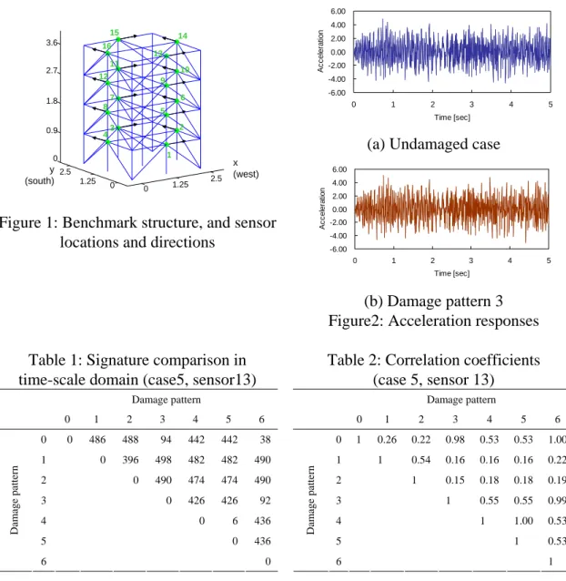
The ASCE Benchmark Problem [9] is used as a test case to show the performance of the damage detection method proposed in this paper. The benchmark structure is a 4-story 2-bay by 2-bay steel frame structure as shown in Fig. 1. MATLAB codes are available on the web site hosted by ASCE Structural Health Monitoring Committee

.

Two finite element models, a 12 degree of freedom (DOF) shear-building model and a 120-DOF model, were developed to generate the simulated response data. Six cases were defined, which had different properties: degrees of freedom; mass distribution; excitation.

Six predefined damage patterns are: (i) no stiffness in the braces in the braces of the first story; (ii) no stiffness in any of the braces of the first and third stories; (iii) no stiffness in one brace in the first story; (iv) no stiffness in one brace in the first story and one brace in the third story; (v) damage pattern (iv) with a floor beam at the first level partially unscrewed;

and (vi) two thirds stiffness in one brace in the first story.

Time-Scale analysis

Only data from the 120-DOF model is used in this paper. Case 5 has an asymmetric mass distribution on the roof and a shaker placed diagonally on the roof. Seven simulations (undamaged and six damaged patterns) with default parameters except for “duration”

modified to 41 seconds were calculated using Nigham-Jennings Algorithm. The response acceleration data is down sampled to 200Hz and the first 8,192 points are analyzed. 256 coefficients are distilled in the signatures, which mean the similarity indices range from 0 to 512. Table 1 shows the results of sensor 13.

Table 1 illustrates the sensitivity for the damage patterns 1, 2, 4 and 5. The damage patterns 3 and 6 are categorized as less severe damage. Also similarities between the damage patterns 4-6, and 3-6 are found.

It seems that Table 1 shows a perfect result to detect damage and to estimate the severities indeed, but almost the same result is derived by calculating correlation coefficients of each pair of the sensor responses as shown in Table 2. The reason is very fundamental; the same external forces are applied to every simulation. Figure 2 displays the time histories of acceleration acquired in the undamaged and the damage pattern 3 computations. No difference between the two signals is distinguished at first glance.

When different seed numbers are used for the input force generation, the signature-based approach cannot detect damage as shown in Table 3. The proposed method exhibits an ability equivalent to that of correlation coefficients with less computation when comparing target and reference signals in time domain analysis.

Frequency-Scale Analysis

It is straightforward to convert time histories of target signals into Fourier coefficients in order to capture the structural behavior. In the following, the performance of frequency-scale domain analysis using Haar wavelet decomposition is explained.

The response acceleration data is down sampled to 200Hz and the first 8,192 points are transferred to 4,096 Fourier amplitudes through FFT. 128 non-zero coefficients are distilled in the signatures, which means the indices may range form 0 to 256.

3

http://cive.seas.wustl.edu/wusceel/asce.shm/

1 3 2

4

5 6 7

8

9 11

12

13 15 14 16

x (west) y

(south)

10

0 0 1.25

1.25 2.5

2.5 0 0.9 1.8 2.7 3.6

Figure 1: Benchmark structure, and sensor locations and directions

-6.00 -4.00 -2.00 0.00 2.00 4.00 6.00

0 1 2 3 4 5

Time [sec]

Acceleration

(a) Undamaged case

-6.00 -4.00 -2.00 0.00 2.00 4.00 6.00

0 1 2 3 4 5

Time [sec]

Acceleration

(b) Damage pattern 3 Figure2: Acceleration responses Table 1: Signature comparison in

time-scale domain (case5, sensor13)

Damage pattern

0 1 2 3 4 5 6 0 0 486 488 94 442 442 38 1 0 396 498 482 482 490 2 0 490 474 474 490 3 0 426 426 92 4 0 6 436

5 0 436

Damage pattern

6 0

Table 2: Correlation coefficients (case 5, sensor 13)

Damage pattern

0 1 2 3 4 5 6

0 1 0.26 0.22 0.98 0.53 0.53 1.00 1 1 0.54 0.16 0.16 0.16 0.22 2 1 0.15 0.18 0.18 0.19 3 1 0.55 0.55 0.99 4 1 1.00 0.53

5 1 0.53

Damage pattern

6 1

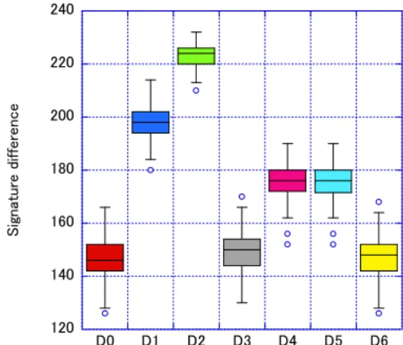
Figure 3 shows the result of frequency-scale domain analysis which means that the acceleration time histories are translated in frequency domain and then the signals in frequency domain are distilled by Haar wavelet decomposition to generate the “signatures”.

Figure 3 illustrates the indices distributions of the predefined damage patterns in comparison with undamaged structure response. A boxplot consists of the largest non-outlier observation, upper quartile (UQ), median, lower quartile (LQ) and smallest non-outlier observation. Outliers are plotted as circle markers. 256 simulations with different seeds for random force generation were performed on each damage pattern including undamaged which denoted D0 in the chart.

Similar trends to Table 1 are obtained. Damage patterns 3 and 6 are categorized as less severe or undamaged in comparison with the distribution of indices under undamaged simulations. The similarities between the damage patterns 4-5, and 3-6 are also found.

Figures 4 to 7 represent the results of sensor 1, 2, 9 and 14 respectively. Damage pattern

3 can be estimated to be less severe through the responses in x-direction (sensors 1, 9 and 13

e.g. Figure 4, 6 and 3). The similarities between the damage patterns 4-5, and 3-6 are found

in the same way with Figure 3.

Table3: Signature comparison of simulations with different seed numbers

Damage pattern (seed #)

0

(123) 1 (31)

2 (61)

3 (251)

4 (17)

5 (7)

6 (191) 0 0 488 508 484 488 506 500 1 0 496 490 494 504 496 2 0 494 496 504 510 3 0 514 496 500 4 0 494 492

5 0 490

Damage pattern

6 0

120 140 160 180 200 220 240 260

D0 D1 D2 D3 D4 D5 D6

Signature difference

Figure 3: Frequency-scale analysis (sensor 13)

120 140 160 180 200 220 240

D0 D1 D2 D3 D4 D5 D6

Signature difference

Figure 4: Frequency-scale analysis (sensor 1)

100 120 140 160 180 200 220 240

D0 D1 D2 D3 D4 D5 D6

Signature difference

Figure 5: Frequency-scale analysis (sensor 2)

120 140 160 180 200 220 240

D0 D1 D2 D3 D4 D5 D6

Signature difference

Figure 6: Frequency-scale analysis (sensor 9)

100 150 200 250

D0 D1 D2 D3 D4 D5 D6

Signature difference

Figure 7: Frequency-scale analysis

(sensor 14)

Some knowledge about damage pattern has been disclosed by combining the results of several sensors without time-synchronization. One sensor source can detect damage pattern 1, 2, 4 and 5 though the investigation of Figures 3-7. That leads to the evidence that damage patterns 1, 2, 4 and 5 are relatively severe. The fact that sensors 1, 9 and 13 cannot detect damage pattern 3 implies that the introduced damage does not affect x-axis properties.

Although the analysis developed in frequency-scale domain requires more computation load before distilling signature, it reduces the volume of data transmission drastically. Also the method proposed in frequency-scale domain analysis does not require time-synchronization of each sensor node.

CONCLUSIONS

A damage detection method using wavelet decomposition was proposed. Through the case study of the ASCE Benchmark Problem, it revealed a potential to skim through huge sensing data. It could compress raw measured data significantly. It could also detect both global and localized damage without time-synchronization of multiple sensor sources.

The algorithm proposed in this paper is simple and fast enough to detect damage and will be a good premise of distributed sensor systems in SHM domain. The case study discloses that only 4 seconds of data sampled at 200Hz 128 signature coefficients are enough to detect all predefined damage cases in frequency-scale analysis.

REFERENCES

1. Lynch, J.P., Sundararajan, A., Law, K.H., Kiremidjian, A.S., and Carryer, E. “Embedding damage detection algorithms in a wireless sensing unit for operational power efficiency.” Smart Materials and Structures, 13: 800-810. (2004)

2. Nagayama, T., Ruiz-Sandoval, M., Spencer Jr., B.F., Mechitov, K.A., and Agha, G. “Wireless Strain Sensor Development for Civil Infrastructure.” Proceedings of First International Workshop on Networked Sensing Systems, Tokyo, Japan, 97-100. (2004)

3. Sohn, H., Farrar, C.R., Hemez, F.M., Shunk, D.D., Stinemates, D.W., and Nadler, B.R. A Review of Structural Health Monitoring Literature: 1996-2001. Los Alamos National Laboratory Report, LA-13976-MS. (2003)

4. Mattson, S.G., and Pandit, S.M. “Statistical moments of autoregressive model residuals for damage localization.” Mechanical Systems and Signal Processing, 20: 627-645. (2006)

5. Sohn, H., Park, G., Wait, J.R., Limback, N.P, and Farrar, C.R. “Wavelet-based active sensing for delamination detection in composite structures.” Smart Materials and Structures, 13: 153-160. (2004) 6. Queck, S.T., Wang, Q., Zhang, L., and Ong, K.H. “Practical issues in the detection of damage in

beams using wavelets.” Smart Materials and Structures, 10: 1009-1017. (2001)

7. Lei, Y., Kiremidjian, A.S., Nair, K.K., Lynch, J.P., and Law, K.H. “Algorithms for time synchronization of wireless structural monitoring sensors.” Earthquake Engineering and Structural Dynamics, 34: 555-573. (2005)

8. Jacobs, C., Finkelstein, A., and Salesin, D. “Fast Multiresolution Image Querying.” SIGGRAPH 95 Proceedings, Annual Conference Series, ACM SIGGRAPH, 277-286. (1995)

9. Johnson, E.A., Lam, H.F., Katafygiotis, L.S., and Beck, J.L. “Phase I IASC-ASCE Structural Health

Monitoring Benchmark Problem Using Simulated Data.” Journal of Engineering Mechanics, ASCE,

130(1): 3-15. (2004)