The construction of numerical schemes for interface problems

The construction of numerical schemes for interface problems

インターフェース問題の数値スキームの 構成（英文）

Department of Mathematics and Information Sciences Graduate School of Science and Engineering

Tokyo Metropolitan University Yingying Wu

首都大学東京大学院理工学研究科数理情報科学専攻 呉 穎穎

2010

Contents

1 Introduction 1

2 One dimensional boundary value problem 3

2.1 The Newton polynomial and Continuity of flux . . . 4

2.1.1 The Newton polynomial . . . 4

2.1.2 Continuity of flux . . . 4

2.2 Four-point finite difference schemes for irregular grid points . . . 5

2.2.1 Main schemes . . . 10

2.2.2 Numerical experiments and results . . . 10

2.3 Six-point finite difference schemes for irregular grid points . . . 12

2.3.1 Main schemes . . . 18

2.3.2 Numerical experiments and results . . . 18

3 Two dimensional elliptic interface problem 25 3.1 First kind of interface . . . 25

3.2 Second kind of interface . . . 29

4 Application of the difference scheme to the evolution equations 34 4.1 One dimensional heat equation . . . 34

4.2 One dimensional wave equation . . . 40

4.3 Two dimensional heat equation . . . 43

4.4 Two dimensional wave equation . . . 48

5 Conclusion 53

Acknowledgement 54

Bibliography 54

Chapter 1 Introduction

Interface problems arise from many applied fields including, for example, the study of two different materials, such as iron and copper, and the same material at different states, such as water and ice. When ordinary or partial differential equations are used to model these applications, the parameters in the governing differential equations are typically dis- continuous across the interface. Because of these irregularities, the solutions to the differ- ential equations are typically nonsmooth, or even discontinuous. As a result, for interface problems many standard numerical methods based on the assumption of smoothness of solutions work poorly or not at all.

For interface problems, analytic solutions are rarely available. The rapid development of modern computers has made it possible to find numerical solutions of these problems.

Standard finite difference methods based on simple grids will likely lead to loss of accuracy in a neighborhood of interfaces. The goal of our presented research is to deal with interface problems and obtain high-order accuracy throughout the entire domain.

Recently, Li and Ito proposed the immersed interface method (IIM) developed for interface problems. This method is based on uniform or adaptive grids or triangulation in Cartesian, polar or spherical coordinates. Standard finite difference or finite element methods are used away from interfaces. The finite difference or finite element schemes are modified locally near or on the interfaces or boundaries according to the interface relations so that high-order accuracy can be obtained in the entire domain.

In this thesis, we will propose new finite difference schemes for interface problems. We will use the Newton polynomial and continuity of flux to obtain the four-point finite difference scheme of first-order accuracy and the six-point finite difference scheme of second-order accuracy at the interface. The resulting numerical methods are easy-to- follow, and the schemes do not rely on Taylor expansions at the interface. The contents of this thesis are as follows:

Chapter 2

In this chapter, we will give the example of one dimensional interface problem. The purpose of this chapter is to analyze this equation. Then we will introduce the Newton polynomial and continuity of flux, which will be used to derive our original four-point

and six-point schemes (instead of Taylor expansion as in IIM by Li-Ito). Numerical experiments and results will be shown respectively. Also we will show the comparison of our schemes with IIM.

Chapter 3

In this chapter, we will give the examples of two dimensional interface problems with two kinds of different interfaces. Our six-point schemes will be used. And we will show the numerical results.

Chapter 4

In this chapter, we will give the application of our six-point schemes to the evolution equations: for the one dimensional heat equation and wave equation with interface; and for the two dimensional heat equation and wave equation with interface.

Chapter 5

We will discuss the results of this thesis.

Chapter 2

One dimensional boundary value problem

In this chapter, we start with the following one-dimensional boundary value problem {

(Bux)x(x) =f(x), a < x < b,

u(a) = C1, u(b) = C2, (2.1)

where the function B(x) is piecewise constant with a discontinuity at x=α (a < α < b).

Reformulating the problem using junction conditions, we obtain











(Bu_x)_x(x) =f(x) x∈(a, α)∪(α, b) [u]_x=α =u⁺−u⁻= 0

[Bu_x]_x=α =B⁺u⁺_x −B⁻u⁻_x = 0 u(a) = C₁, u(b) = C₂.

(2.2)

Remark 1. If f(x) ∈ C²((a, α])∩C²([α, b)), even if f(x) is discontinuous at α, then u(x)∈C⁴((a, α])∩C⁴([α, b)) and u(x) is Lipschitz continuous.

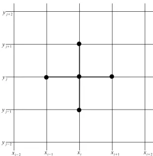
After generating a Cartesian grid, say xi = ih, i = 0,1,· · · , N, where h = (b − a)/(N + 1), the point α will fall on a single grid point or between two grid points, that is, x_j ≤ α < x_j+1. The grid points x_j and x_j+1 (see Figure 2.1) are called irregular grid points. All other grid points are called regular grid points, where the standard 3-point central finite difference stencil

1 h²(B_i+¹

2(U_i+1−U_i)−B_i−¹

2(U_i−U_i−1)) =f_i is used here, noting that B_i+¹

2 = B(x_i+¹

2) and f_i = f(x_i). The problem is then to find suitable difference equations for the irregular grid points, x_j and x_j+1.

Figure 2.1: A one-dimensional grid with the interface α between grid points x_j and x_j+1.

2.1 The Newton polynomial and Continuity of flux

2.1.1 The Newton polynomial

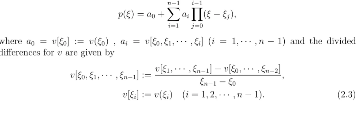
To determine the difference equations at the irregular grid points, we firstly introduce Newton’s interpolation (extrapolation), see for example [1]. For a given smooth function v(ξ), Newton’s interpolation is defined by:

p(ξ) =a₀+

n−1

∑

i=1

a_i

i−1

∏

j=0

(ξ−ξ_j),

where a₀ = v[ξ₀] := v(ξ₀) , a_i = v[ξ₀, ξ₁,· · · , ξ_i] (i = 1,· · · , n − 1) and the divided differences for v are given by

v[ξ₀, ξ₁,· · · , ξ_n−1] := v[ξ₁,· · · , ξ_n−1]−v[ξ₀,· · · , ξ_n−2] ξ_n−1−ξ₀ ,

v[ξi] :=v(ξi) (i= 1,2,· · · , n−1). (2.3)

2.1.2 Continuity of flux

Let us consider the general case where f(x) is assumed to be smooth in (−∞, α] and [α,∞).

Lemma 1. If f(x)∈C²((−∞, α])∩C²([α,∞)), we have B⁺ux(xj+1)−B⁻ux(xj−1) =−h

2((d²−1)fj−1−(d+ 1)²fj−(d−1)(d−3)fj+1+ (d−1)²fj+2) +O(h³), (2.4)

B⁺u_x(x_j+2)−B⁻u_x(x_j) =−h

2(d²f_j−1−d(d+ 2)f_j−(d−2)²f_j+1+d(d−2)f_j+2) +O(h³).

(2.5) Proof. For the irregular point x_j, we have

B⁺u_x(x_j+1)−B⁻u_x(x_j−1) =

∫ xj+1

xj−1

f(x)dx=

∫ α xj−1

f(x)dx+

∫ xj+1

α

f(x)dx

=

∫ α xj−1

(

f[xj] +f[xj, xj−1](x−xj) )

dx+

∫ xj+1

α

(

f[xj+1] +f[xj+1, xj+2](x−xj+1) )

dx+O(h³)

= (α−x_j−1)f_j+ fj−fj−1

h · (α−xj)² −h²

2 + (x_j+1−α)f_j+1− fj+2−fj+1

h ·(α−xj+1)²

2 +O(h³)

=−h

2(d²−1)fj−1+ h

2(d+ 1)²fj+ h

2(d−1)(d−3)fj+1− h

2(d−1)²fj+2+O(h³).

Similarly, for x_j+1, we have

B⁺u_x(x_j+2)−B⁻u_x(x_j) =

∫ _xj+2

xj

f(x)dx =

∫ _α

xj

f(x)dx+

∫ _xj+2

α

f(x)dx

=

∫ α xj

(

f[x_j] +f[x_j, x_j−1](x−x_j) )

dx+

∫ xj+2

α

(

f[x_j+1] +f[x_j+1, x_j+2](x−x_j+1) )

dx+O(h³)

= (α−x_j)f_j+ f_j −f_j−1

h · (α−x_j)²

2 + (x_j+2−α)f_j+1+f_j+2−f_j+1

h · h²−(α−x_j+1)²

2 +O(h³)

=−h

2d²f_j−1+h

2d(d+ 2)f_j +h

2(d−2)²f_j+1− h

2d(d−2)f_j+2+O(h³).

2.2 Four-point finite difference schemes for irregular grid points

The expected four-point finite difference equations are determined from the method of undetermined coefficients,

γ_j−1U_j−1+γ_jU_j+γ_j+1U_j+1+γ_j+2U_j+2 =f_j, δ_j−1U_j−1+δ_jU_j +δ_j+1U_j+1+δ_j+2U_j+2 =f_j+1.

Applying the Newton polynomial with n = 3 to v(ξ), for ξ ≥ α, with ξ0, ξ1 and ξ2

replaced respectively by ξ_j+1, ξ_j+2 and ξ_j+3 we obtain

p⁺(ξ) =v(ξ_j+1) +v[ξ_j+1, ξ_j+2](ξ−ξ_j+1) +v[ξ_j+1, ξ_j+2, ξ_j+3](ξ−ξ_j+1)(ξ−ξ_j+2)

=v(ξ_j+1) + v(ξ_j+2)−v(ξ_j+1)

h (ξ−ξ_j+1) + v(ξ_j+3)−2v(ξ_j+2) +v(ξ_j+1)

2h² (ξ−ξ_j+1)(ξ−ξ_j+2)

=v(ξ_j+1) (

1− ξ−ξ_j+1

h +(ξ−ξ_j+1)(ξ−ξ_j+2) 2h²

)

+v(ξ_j+2)

(ξ−ξ_j+1

h − (ξ−ξ_j+1)(ξ−ξ_j+2) h²

)

+v(ξ_j+3)

((ξ−ξ_j+1)(ξ−ξ_j+2) 2h²

) ,

where the superscript + in p⁺(ξ) indicates an expansion on the right hand side, that is,

ξ ≥α. This gives a higher order approximation of v(α). Similarly, forξ ≤α, we obtain p⁻(ξ) =v(ξ_j) +v[ξ_j, ξ_j−1](ξ−ξ_j) +v[ξ_j, ξ_j−1, ξ_j−2](ξ−ξ_j)(ξ−ξ_j−1)

=v(ξ_j) + v(ξ_j)−v(ξ_j−1)

h (ξ−ξ_j) + v(ξ_j)−2v(ξ_j−1) +v(ξ_j−2)

2h² (ξ−ξ_j)(ξ−ξ_j−1)

=v(ξ_j) (

1 + ξ−ξ_j

h + (ξ−ξ_j)(ξ−ξ_j−1) 2h²

)

+v(ξ_j−1) (

−ξ−ξ_j

h − (ξ−ξ_j)(ξ−ξ_j−1) h²

)

+v(ξ_j−2)

((ξ−ξ_j)(ξ−ξ_j−1) 2h²

) ,

where the superscript − in p⁻(ξ) indicates an expansion on the left hand side, that is, ξ ≤α. This again gives a higher order approximation of v(α).

Differentiating both p⁺(ξ) (ξ≥α) andp⁻(ξ) (ξ≤α) with respect to ξ, we have p⁺_ξ(ξ) = 1

h (

v(ξ_j+2)−v(ξ_j+1) )

+ 1 2h²

(

v(ξ_j+3)−2v(ξ_j+2)+v(ξ_j+1) )

(2ξ−ξ_j+1−ξ_j+2), (2.6)

p⁻_ξ(ξ) = 1 h

(

v(ξj)−v(ξj−1) )

+ 1 2h²

(

v(ξj)−2v(ξj−1) +v(ξj−2) )

(2ξ−ξj −ξj−1), (2.7) and hence obtain higher order approximations of v_ξ(α), thanks to the following basic result on the polynomial interpolation (eg. [1] p. 56 Theorem 3.1.1).

Lemma 2. For ξ_i(0 ≤i ≤ 2)∈(a, b), let p(ξ) be the second-order Newton interpolation of v(ξ). If v(ξ)∈C³(a, b), then there exists an η such that

v(ξ)−p(ξ) = v⁽³⁾(η)

3! (ξ−ξ0)(ξ−ξ1)(ξ−ξ2), where min(ξ, ξ₀, ξ₁, ξ₂)< η <max(ξ, ξ₀, ξ₁, ξ₂).

Note that from this lemma we can derive immediately the following proposition.

Proposition 1. If v ∈ C³((−∞, α])∩ C³([α,∞)), then for ξ = α + O(h), we have v(ξ)−p(ξ) = O(h³), where p(ξ) =p⁺(ξ) for ξ > α, p(ξ) =p⁻(ξ) for ξ < α.

Similarly, Lemma 2 yields the following estimate for the derivative of v−p in view of the Rolle’s theorem.

Proposition 2. If v ∈ C³((−∞, α])∩ C³([α,∞)), then for ξ = α + O(h), we have v_ξ(ξ)−p_ξ(ξ) = O(h²), where p_ξ(ξ) =p⁺_ξ(ξ) for ξ > α, p_ξ(ξ) = p⁻_ξ(ξ) for ξ < α.

Let us define

d:= α−x_j h .

Remark 2. 0≤d <1.

Corollary 1. Assume thatf(x)∈C²((−∞, α])∩C²([α,∞))and let u(x)be the solution of (2.2). Then we have

(i)

u(α⁺) =u(x_j+1) (

1−α−x_j+1

h + (α−x_j+1)(α−x_j+2) 2h²

)

+u(x_j+2)

(α−x_j+1

h − (α−x_j+1)(α−x_j+2) h²

)

+u(x_j+3)

((α−x_j+1)(α−x_j+2) 2h²

)

+O(h³)

= 1

2(d−2)(d−3)u(x_j+1)−(d−1)(d−3)u(x_j+2) + 1

2(d−1)(d−2)u(x_j+3) +O(h³), (ii)

u(α⁻) = u(x_j) (

1 + α−x_j

h + (α−x_j)(α−x_j−1) 2h²

)

+u(x_j−1) (

−α−x_j

h − (α−x_j)(α−x_j−1) h²

)

+u(x_j−2)

((α−x_j)(α−x_j−1) 2h²

)

+O(h³)

= 1

2(d+ 1)(d+ 2)u(x_j)−d(d+ 2)u(x_j−1) + 1

2d(d+ 1)u(x_j−2) +O(h³), (iii)

u_x(α⁺) =− 1

2h(2d−5)u(x_j+1)− 1

h(2d−4)u(x_j+2) + 1

2h(2d−3)u(x_j+3) +O(h²), (iv)

u_x(α⁻) = 1

2h(2d+ 3)u(x_j)− 1

2(2d+ 2)u(x_j−1) + 1

2h(2d+ 1)u(x_j−2) +O(h²).

Substitutingu(α⁺), u(α⁻), u_x(α⁺) andu_x(α⁻) for the junction conditions in (2.2), and letting u_j =u(x_j), we obtain

d(d+ 1)u_j−2−2d(d+ 2)u_j−1+ (d+ 1)(d+ 2)u_j

= (d−2)(d−3)uj+1−2(d−1)(d−3)uj+2+ (d−1)(d−2)uj+3+O(h³), (2.8)

B⁻(2d+ 1)u_j−2 −2B⁻(2d+ 2)u_j−1+B⁻(2d+ 3)u_j

=B⁺(2d−5)u_j+1−2B⁺(2d−4)u_j+2+B⁺(2d−3)u_j+3+O(h³). (2.9)

From (2.8) and (2.9), we have u_j+3=− 1

P_j+3(P_j−1u_j−1 +P_ju_j +P_j+1u_j+1+P_j+2u_j+2) +O(h³), (2.10) u_j−2 =− 1

Q_j−2(Q_j−1u_j−1+Q_ju_j+Q_j+1u_j+1+Q_j+2u_j+2) +O(h³), (2.11) where

P_j−1 =−2B⁻d², P_j = 2B⁻(d+ 1)²,

P_j+1 =−B⁻(d−2)(d−3)(2d+ 1) +B⁺d(d+ 1)(2d−5), P_j+2 = 2B⁻(d−1)(d−3)(2d+ 1)−2B⁺d(d+ 1)(2d−4), Pj+3 =−B⁻(d−1)(d−2)(2d+ 1) +B⁺d(d+ 1)(2d−3), and

Q_j−2 =B⁺d(d+ 1)(2d−3)−B⁻(d−1)(d−2)(2d+ 1), Q_j−1 =−2B⁺d(d+ 2)(2d−3) + 2B⁻(d−1)(d−2)(2d+ 2)),

Q_j =B⁺(d+ 1)(d+ 2)(2d−3)−B⁻(d−1)(d−2)(2d+ 3), Q_j+1 = 2B⁺(d−2)²,

Qj+2 =−2B⁺(d−1)².

Remark 3. P_j+3 =Q_j−2 and |P_j+3| is bounded above 0 uniformly for 0≤d <1.

Using the approximation (2.6) for u(x) at x_j+1 and x_j+2, and (2.7) for u(x) at x_j−1 and x_j, we get

u_x(x_j+1) = 1

2h(−3u_j+1+ 4u_j+2−u_j+3) +O(h²), u_x(x_j+2) = 1

2h(−u_j+1+u_j+3) +O(h²), u_x(x_j−1) = 1

2h(−u_j−2+u_j) +O(h²), u_x(x_j) = 1

2h(u_j−2−4u_j−1+ 3u_j) +O(h²).

Substituting the above four equations in (2.4) and (2.5), we obtain B⁺

2h(−3u_j+1+ 4u_j+2−u_j+3)− B⁻

2h(−u_j−2+u_j)

=−h

2(d²−1)f_j−1+h

2(d+ 1)²f_j +h

2(d−1)(d−3)f_j+1− h

2(d−1)²f_j+2+O(h³), (2.12)

B⁺

2h(−u_j+1+u_j+3)− B⁻

2h(u_j−2−4u_j−1+ 3u_j)

=−h

2d²fj−1+ h

2d(d+ 2)fj+ h

2(d−2)²fj+1−h

2d(d−2)fj+2+O(h³). (2.13) We replace fj−1 and fj+2 in the right hand sides of (2.12) and (2.13) by

fj−1 =B⁻u_j−2−2u_j−1+u_j

h² +O(h²), f_j+2 =B⁺u_j+1−2u_j+2+u_j+3

h² +O(h²).

Therefore, f_j and f_j+1 can be approximately expressed as linear combinations of u_i, i=j−2,· · · , j+ 3. The results are

B⁻ (

(2d²−4d+ 3)u_j−2−2(2d²−4d+ 2)u_j−1+ (2d² −4d+ 1)u_j )

+B⁺ (

(2d−5)u_j+1−2(2d−4)u_j+2+ (2d−3)u_j+3 )

= 2(d²−d+ 2)h²f_j +O(h³),

B⁻ (

(2d+ 1)u_j−2−2(2d+ 2)u_j−1+ (2d+ 3)u_j )

+B⁺ (

−(2d²−1)u_j+1+ 4d²u_j+2−(2d² + 1)u_j+3 )

=−2(d²−d+ 2)h²f_j+1+O(h³).

Substituting (2.10) and (2.11) in the above two equations, we obtain γ_j−1 = B⁻

h² (

−2−Q_j−1 Q_j−2

)

, γ_j = B⁻ h²

(

1− Q_j Q_j−2

)

, γ_j+1 = B⁻ h²

(

−Q_j+1 Q_j−2

)

, γ_j+2 = B⁻ h²

(

−Q_j+2 Q_j−2

) , and

δ_j−1 = B⁺ h²

(

−P_j−1 P_j+3

)

, δ_j = B⁺ h²

(

− P_j P_j+3

)

, δ_j+1 = B⁺ h²

(

1−P_j+1 P_j+3

)

, δ_j+2 = B⁺ h²

(

−2−P_j+2 P_j+3

) , Remark 4. Whenα is at the mid-point of the interval [a, b], i.e., α= ^a+b₂ , takingB⁻ = 1 and B⁺ = 2, we have

γ_j−1 = 11 9

1

h², γ_j =− 3

h², γ_j+1 = 2

h², γ_j+2 =−2 9

1 h², δ_j−1 =−2

9 1

h², δ_j = 2

h², δ_j+1 =− 4

h², δ_j+2 = 20 9

1 h², which will be used later in our numerical examples.

2.2.1 Main schemes

Finally we arrive at the following theorem.

Theorem 1. Let f satisfy the same assumption as in Lemma 1. Then, if u is the so- lution of (2.1), the following finite differences are respectively equal to (Bu_x)_x(x_j) and (Bu_x)_x(x_j+1) up to O(h).

γ_j−1u_j−1+γ_ju_j +γ_j+1u_j+1+γ_j+2u_j+2, δ_j−1u_j−1+δ_ju_j +δ_j+1u_j+1+δ_j+2u_j+2, where γ_i and δ_i(i=j −1,· · · , j+ 2) are given above.

Corollary 2. The expected finite difference schemes can be obtained by replacing u_j, u_j+1 with U_j, U_j+1 and (Bu_x)_x(x_j), (Bu_x)_x(x_j+1) with f_j, f_j+1,

γ_j−1U_j−1+γ_jU_j+γ_j+1U_j+1+γ_j+2U_j+2 =f_j, δ_j−1U_j−1+δ_jU_j +δ_j+1U_j+1+δ_j+2U_j+2 =f_j+1. Remark 5. Naturally, for the regular grid pointsx_i (i̸=j, j + 1),

Bu_i+1−2u_i+u_i−1

h² = (Bu_x)_x(x_i) +O(h²).

Remark 6. When the point α falls on a grid point, for example, on x_j, x_j will be the only irregular grid point. Further, at x_j a four-point scheme will be used , and at x_j+1 the scheme is reduced to the usual 3-point central difference scheme since δ_j−2, δ_j−1 and δ_j+3 vanish.

2.2.2 Numerical experiments and results

Let us compute numerical solution in the following case (Bux)x(x) = 12x² B =

{

B⁻ x <0.5, B⁺ x >0.5, u(0) = 0, u(1) = 1.

Heref(x)∈C²(0,1) and the natural jump conditions [u] = 0 and [Bu_x] = 0 are satisfied across the interface α. The exact solution is given by

u(x) =





x⁴

B⁻ x < α,

x⁴ B⁺ +

(

1 B⁻ − _B¹+

)

α⁴ x > α.

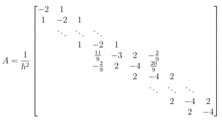
If we take α = 1/2(= (x_j +x_j+1)/2), B⁻ = 1, B⁺ = 2, and apply our four-point schemes to this problem, we obtain a linear system ofN equations for N unknowns, which can be written in the form

AU =F, (2.14)

where U is the vector of unknowns, U = [U₁, U₂,· · · , U_N]^T,

A= 1 h²



















−2 1 1 −2 1

. .. ... ...

1 −2 1

11

9 −3 2 −²₉

−²₉ 2 −4 ²⁰₉ 2 −4 2

. .. ... ...

2 −4 2 2 −4

















 ,

noting that the values of γ and δ were given in Remark 4, and

F =











12x²₁ 12x²₂ 12x²₃

... 12x²_N−1 12x²_N −17/32









 .

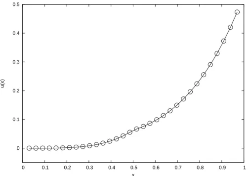
Computing this linear system, we get a numerical solution which is indistinguishable from the exact solution, see Figure 2.2. Table 2.1 shows the results of a grid refinement analysis, where the absolute error is measured using the L^∞ and L² norms,

∥E_N∥_∞= max

i |u(x_i)−U_i|,

∥E_N∥L² =

√1 N

∑

i

|u(x_i)−U_i|².

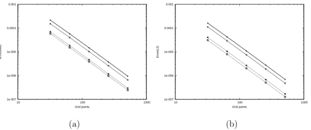
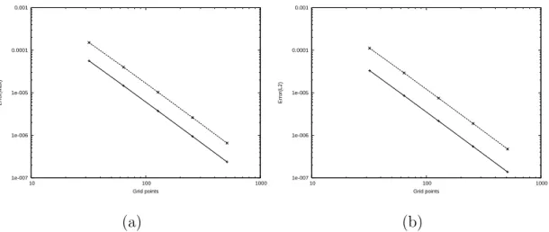
Figure 2.3 depicts the double logarithmic plots of∥E_N∥_∞and∥E_N∥L², withN = 32,64,128,256 and 512, which shows that the ratio ∥E_N∥∞/∥E_2N∥∞ approaches 4 as N increases, in- dicating that our four-point method yields the error of second-order for this particular model.

Table 2.1: Grid refinement analysis with α= 1/2, B⁻ = 1 andB⁺ = 2.

N 32 64 128 256 512

∥E_N∥_∞ 1.618×10⁻⁴ 4.063×10⁻⁵ 1.017×10⁻⁵ 2.592×10⁻⁶ 6.551×10⁻⁷

∥E_N∥L² 1.138×10⁻⁴ 2.950×10⁻⁵ 7.517×10⁻⁶ 1.897×10⁻⁶ 4.767×10⁻⁷

0 0.1 0.2 0.3 0.4 0.5

0 0.1 0.2 0.3 0.4 0.5 0.6 0.7 0.8 0.9 1

u(x)

x

Figure 2.2: Comparison of the computed solution (circles) and exact solution (solid line).

1e-007 1e-006 1e-005 0.0001 0.001

10 100 1000

Error(Max)

Grid points

(a)

1e-007 1e-006 1e-005 0.0001 0.001

10 100 1000

Error(L2)

Grid points

(b)

Figure 2.3: Double logarithmic plots of (a) ∥E_N∥_∞ and (b) ∥E_N∥L².

2.3 Six-point finite difference schemes for irregular grid points

The expected six-point finite difference equations are determined from the method of undetermined coefficients,

γ_j−2U_j−2+γ_j−1U_j−1+γ_jU_j+γ_j+1U_j+1+γ_j+2U_j+2+γ_j+3U_j+3 =f_j, δj−2Uj−2+δj−1Uj−1+δjUj+δj+1Uj+1+δj+2Uj+2+δj+3Uj+3 =fj+1.

Applying the Newton polynomial with n = 4 to v(ξ), for ξ ≥ α, with ξ₀, ξ₁, ξ₂ and

ξ₃ replaced respectively by ξ_j+1, ξ_j+2, ξ_j+3 and ξ_j+4 in the same way as last section, we obtain

p⁺(ξ) =v(ξ_j+1) +v[ξ_j+1, ξ_j+2](ξ−ξ_j+1) +v[ξ_j+1, ξ_j+2, ξ_j+3](ξ−ξ_j+1)(ξ−ξ_j+2) +v[ξ_j+1, ξ_j+2, ξ_j+3, ξ_j+4](ξ−ξ_j+1)(ξ−ξ_j+2)(ξ−ξ_j+3)

=v(ξ_j+1) + v(ξ_j+2)−v(ξ_j+1)

h (ξ−ξ_j+1) + v(ξ_j+3)−2v(ξ_j+2) +v(ξ_j+1)

2h² (ξ−ξ_j+1)(ξ−ξ_j+2) +v(ξ_j+4)−3v(ξ_j+3) + 3v(ξ_j+2)−v(ξ_j+1)

6h³ (ξ−ξ_j+1)(ξ−ξ_j+2)(ξ−ξ_j+3)

=v(ξ_j+1) (

1− ξ−ξ_j+1

h +(ξ−ξ_j+1)(ξ−ξ_j+2)

2h² − (ξ−ξ_j+1)(ξ−ξ_j+2)(ξ−ξ_j+3) 6h³

)

+v(ξ_j+2)

(ξ−ξ_j+1

h − (ξ−ξ_j+1)(ξ−ξ_j+2)

h² +(ξ−ξ_j+1)(ξ−ξ_j+2)(ξ−ξ_j+3) 2h³

)

+v(ξ_j+3)

((ξ−ξ_j+1)(ξ−ξ_j+2)

2h² − (ξ−ξ_j+1)(ξ−ξ_j+2)(ξ−ξ_j+3) 2h³

)

+v(ξ_j+4)

((ξ−ξ_j+1)(ξ−ξ_j+2)(ξ−ξ_j+3) 6h³

) ,

where the superscript + in p⁺(ξ) indicates an expansion on the right hand side, that is, ξ ≥α. This gives a higher order approximation of v(α). Similarly, forξ ≤α, we obtain

p⁻(ξ) =v(ξ_j) +v[ξ_j, ξ_j−1](ξ−ξ_j) +v[ξ_j, ξ_j−1, ξ_j−2](ξ−ξ_j)(ξ−ξ_j−1) +v[ξ_j, ξ_j−1, ξ_j−2, ξ_j−3](ξ−ξ_j)(ξ−ξ_j−1)(ξ−ξ_j−2)

=v(ξ_j) + v(ξ_j)−v(ξ_j−1)

h (ξ−ξ_j) + v(ξ_j)−2v(ξ_j−1) +v(ξ_j−2)

2h² (ξ−ξ_j)(ξ−ξ_j−1) +v(ξ_j)−3v(ξ_j−1) + 3v(ξ_j−2)−v(ξ_j−3)

6h³ (ξ−ξ_j)(ξ−ξ_j−1)(ξ−ξ_j−2)

=v(ξj) (

1 + ξ−ξ_j

h + (ξ−ξ_j)(ξ−ξ_j−1)

2h² + (ξ−ξ_j)(ξ−ξ_j−1)(ξ−ξ_j−2) 6h³

)

+v(ξj−1) (

−ξ−ξ_j

h − (ξ−ξ_j)(ξ−ξ_j−1)

h² − (ξ−ξ_j)(ξ−ξ_j−1)(ξ−ξ_j−2) 2h³

)

+v(ξj−2)

((ξ−ξ_j)(ξ−ξ_j−1)

2h² + (ξ−ξ_j)(ξ−ξ_j−1)(ξ−ξ_j−2) 2h³

)

+v(ξj−3) (

−(ξ−ξ_j)(ξ−ξ_j−1)(ξ−ξ_j−2) 6h³

) ,

where the superscript − in p⁻(ξ) indicates an expansion on the left hand side, that is, ξ ≤α. This again gives a higher order approximation of v(α).

Differentiating both p⁺(ξ) (ξ≥α) andp⁻(ξ) (ξ≤α) with respect to ξ, we have p⁺_ξ(ξ) = 1

h (

v(ξ_j+2)−v(ξ_j+1) )

+ 1 2h²

(

v(ξ_j+3)−2v(ξ_j+2) +v(ξ_j+1) )

(2ξ−ξ_j+1−ξ_j+2) + 1

6h³ (

v(ξ_j+4)−3v(ξ_j+3) + 3v(ξ_j+2)−v(ξ_j+1) )(

(ξ−ξ_j+2)(ξ−ξ_j+3) + (ξ−ξ_j+1) (ξ−ξ_j+3) + (ξ−ξ_j+1)(ξ−ξ_j+2)

) ,

(2.15) p⁻_ξ(ξ) = 1

h (

v(ξ_j)−v(ξ_j−1) )

+ 1 2h²

(

v(ξ_j)−2v(ξ_j−1) +v(ξ_j−2) )

(2ξ−ξ_j −ξ_j−1) + 1

6h³ (

v(ξ_j)−3v(ξ_j−1) + 3v(ξ_j−2)−v(ξ_j−3) )(

(ξ−ξ_j−1)(ξ−ξ_j−2) + (ξ−ξ_j) (ξ−ξ_j−2) + (ξ−ξ_j)(ξ−ξ_j−1)

) ,

(2.16) and hence obtain higher order approximations of v_ξ(α), thanks to the following basic result on the polynomial interpolation (eg. [1] p. 56 Theorem 3.1.1).

Lemma 3. For ξ_i(0≤i≤3)∈(a, b), let p(ξ) be the third-order Newton interpolation of v(ξ). If v(ξ)∈C⁴(a, b), then there exists an η such that

v(ξ)−p(ξ) = v⁽⁴⁾(η)

4! (ξ−ξ₀)(ξ−ξ₁)(ξ−ξ₂)(ξ−ξ₃), where min(ξ, ξ₀, ξ₁, ξ₂, ξ₃)< η <max(ξ, ξ₀, ξ₁, ξ₂, ξ₃).

Note that from this lemma we can derive immediately the following proposition.

Proposition 3. If v ∈ C⁴((−∞, α])∩ C⁴([α,∞)), then for ξ = α + O(h), we have v(ξ)−p(ξ) = O(h⁴), where p(ξ) =p⁺(ξ) for ξ > α, p(ξ) =p⁻(ξ) for ξ < α.

Similarly, Lemma 3 yields the following estimate for the derivative of v−p in view of the Rolle’s theorem.

Proposition 4. If v ∈ C⁴((−∞, α])∩ C⁴([α,∞)), then for ξ = α + O(h), we have v_ξ(ξ)−p_ξ(ξ) = O(h³), where p_ξ(ξ) =p⁺_ξ(ξ) for ξ > α, p_ξ(ξ) = p⁻_ξ(ξ) for ξ < α.

Corollary 3. Assume thatf(x)∈C²((−∞, α])∩C²([α,∞))and let u(x)be the solution of (2.2). Then we have

(i)