Ross Recovery under the Tree Model and Its Application to Risk Management

(1)

TOKYO METROPOLITAN UNIVERSITY

Ross Recovery under the Tree Model and Its Application to Risk Management

by

Koji Anamizu

A thesis submitted in fulfillment for the degree of Master of Finance

Department of Business Administration Graduate School of Social Sciences

January 10th, 2018

(2)

Abstract

Ross (2015) has shown that real-world distributions can be derived from risk-neutral densities, named the Recovery Theorem, which makes the information embedded in option prices directly accessible to applications such as trading strategies, portfolio optimization and risk management. However, as we have to solve an ill-posed problem in the recovery process, application of the theorem to empirical problems is not straightforward. We propose a new method based on the trinomial tree model. Under the method, in addition to its accuracy and robustness, we can decrease the computational time drastically. We then apply the method to the stock and FX markets. By using the recovered real-world distribution, we create some early warning indicators to predict the future risk events, and show their eﬀectiveness.

Keywords: Recovery theorem, physical distribution, tree model, risk management, early warning indicator, forward-looking approach

(3)

Acknowledgment

First, my deepest appreciation goes to Professor Masaaki Kijima of Master of Finance Program, Tokyo Metropolitan University. Without his guidance and persistent help, this thesis would not have been possible. His comments and suggestions were ines- timable value for my study. I also have greatly benefited from Eri Nakamura and Hitomi Ito. As the member in the same laboratory, they always gave me constructive comments and also they checked my presentation paper. In addition, I appreciate my company’s supervisors for giving me a chance to study at the university and their financial support. Finally, I would like to express my gratitude to my family for their moral support and warm encouragement.

(4)

Chapter 1 Introduction

The quality required in the risk management has changed significantly after the global financial crisis in 2008. Major Banks have been forced to develop new risk management tools to supplement the traditional risk measures such as Value at Risk (VaR). In this chapter, we explain the current environment of banks’ risk management and popular risk-measures’ drawbacks.

1.1 Risk Management after the Global Financial Crisis

The global financial crisis highlighted global regulatory weaknesses. After the crisis, a lot of regulations’ changes were considered and actually executed by Basel Commit- tee on Banking Supervision (BCBS) and other financial regulators such as Federal Reserve, European Banking Authority and Bank of England. The event showed us that there were too little liquidity and capital in the banking system. Furthermore, lacking foresight in risk management and delay of the loss recognition were recognized as one of the biggest issues among regulators and banks. The main reason why such problems happened was that banks had heavily depended only on the historical-based approach like VaR (i.e. backward-looking approach). Hence, they have proposed sev- eral methods in the field of risk management to incorporate the foreseeable future into their risks.

Implementation of the Forward-Looking Approach

For example, stress testing is becoming the major risk management tool to cover the traditional risk indicators’ drawback. The main objective of stress testing is to capture the foreseeable scenario (i.e. forward-looking approach), which might be going to happen with high probability or aﬀect negatively on their business. Before the crisis,

(7)

for supervisors, stress testing was ad hoc tool to assess the current state of their domes- tic banking industry in the aftermath of severe external shocks. Increasingly, however, they are becoming regular features of the ongoing regulatory process. Also, for banks, the importance of stress testing is increasing as well. Especially, banks operating inter- nationally, so-called Global-Systemically-Important-Banks (G-SIBs), are facing more comprehensive stress testing requirements. Actually, current tests are placing greater emphasis on both qualitative and quantitative analysis to evaluate broader risks within banks, though initial stress testing exercises mainly focused only on quantitative indicators like the capital ratio.

In addition, in the accounting field, a new allowance calculation method, expected- credit-loss (ELS), was proposed in International Financial Reporting Standards (IFRS).

Before 2008, incurred-loss-model served as the basis for accounting recognition and measurement of credit losses. Under incurred-loss-model, banks were required only certain period’s expected loss calculated mainly by the historical loss data. On the other hand, ELS requires banks to take their future scenarios into account the calculation of the allowance. In general, ELS increases the amount of banks’ allowance and also the implementation cost is expected to be very large because current banks’ accounting systems need many improvements to deal with this new method. Therefore, this change is still a big issue among them.

Stress Testing

Using the United States’ supervisory stress testing as the example, which is known as comprehensive capital analysis and review or CCAR, we explain the basic of stress testing framework.

CCAR is the United States regulatory framework introduced by the Federal Reserve to assess, regulate and supervise large banks. CCAR is executed once a year. The assessment is performed on both qualitative and quantitative basis. In the assessment on the quantitative basis, common-equity-tier-1 and tier-1-leverage-ratio are mainly used to check whether banks’ capital structures are stable given the stress testing scenarios and also whether the planned capital distributions are viable and acceptable.

On the qualitative basis, on the other hand, Federal Reserve recently focuses on wide range of topics such as methods of banks’ internal risk management, model risks, and capital planning processes. If they fail to pass the minimum requirements, they are forced to change their next year’s business plans, including dividend plans and investment strategies. Therefore, banks now spend a high amount of time and money on this program. Figure 1.1 is the process image of stress testing.

(8)

Figure 1.1: process image of stress testing

After preparing the data sets and developing each category’s stress testing model, banks communicate internally and externally and decide the macro scenarios that im- pact significantly their business plans. Then they put the scenarios into the models to estimate the future profit, capital ratio and so on. In the case of CCAR, Federal Reserve investigates the result of the numerical test, its process, models, scenarios and current risk management framework to judge whether a bank passes the requirements or not.

1.2 Main Theme of the Thesis

Unfortunately, we can not say both stress testing and ELS are perfect forward- looking approaches. In most cases, the models used in the stress testing and ELS are based on the historical data. Therefore, when an event which has not occurred before happens, it is almost impossible to predict it beforehand. Moreover, scenarios used in the stress testing and ELS basically depend on economists’ expert judgments or past historical events like Black Monday in 1987 and LTCM crisis in 1998, and also all foreseeable future scenarios are, of course, not included in stress testing.

To cover these drawbacks, banks are developing forward-looking indicators (i.e., early warning indicator (EWI)). Some of them are actually being used among practi- tioners. However, these indicators don’t have robust theoretical backgrounds, and also their quality is generally not so high.

The aim of this thesis is to develop a better EWI not relying on the historical data. We consider to use the option data quoted on the market. The payoﬀ of option is determined by the future distribution of underlying asset price and therefore the option prices contain the forward looking information. It can be expected that it is useful for predicting the future market condition. However, pricing the option value is done under risk-neutral measure which includes risk premium. So, we can’t use the option data straightforwardly. Ross (2015) shows the real-world distributions can

(9)

be derived from risk-neutral densities, named the Recovery Theorem, which makes the information embedded in option prices directly accessible to applications such as trading strategies, portfolio optimization and risk management. In this thesis, by using the theorem, we recover the physical distribution and find the eﬀective indicators that can predict the future market condition.

Structure of the Thesis

This thesis proceeds as follows. Chapter 2 summarizes the Recovery Theorem and how to apply it to real data. In addition, we also explain basic framework of the asset pricing theory as the reference. Moreover, we explain a problem the theorem has (ill-posed problem). Chapter 3 proposes a new approach (tree approach) to cope with the ill-posed problem. We also show its high accuracy and fast computation speed by comparing it with other approaches. Chapter 4 applies the tree approach to risk management. We apply it to S&P500 and USDJPY, and we recover their physical distributions. Then, we create EWI candidates and check each one’s power for predicting the future risk event. In the final chapter, we conclude and describe future works.

(10)

Chapter 2 Asset Pricing Theory and the Recovery Theorem

In this chapter, we explain the basic framework of the asset pricing theory and the recovery theorem. After that, we introduce the literature related to the theorem.

2.1 Framework of the Asset Pricing Theory

In the framework of the asset pricing theory, a state price is an imaginary security price which brings a unit payoﬀ when a certain state happens. This state price is determined uniquely under the assumption of an arbitrage-free and complete market.

Define economic condition at time s as θ_s, s ∈ [t, T] and its state price at time T as p(θ_T|θ_t). The time-t price of the securityv_t can be expressed as

v_t =

∫

g(θ_T)p(θ_T|θ_t)dθ_T, (2.1) where g(θ_T) is a payoﬀ function in the state θ_T. The sum of the state prices coincides with the zero-coupon bond price as

e^−r(θ^t^)T =

∫

p(θ_T|θ_t)dθ_T, (2.2)

where r(θ_t) describes a risk-free-rate function in the stateθ_t. Normalized p(θ_T|θ_t) satisfies the characteristics of the probability, and it is called the risk-neutral probability.

By using (2.2), risk-neutral density q(θ_T|θ_t) can be expressed as follows:

q(θ_T|θ_t) ≡ p(θ_T|θ_t)

∫ p(θT|θt)dθT

, (2.3)

= e^r(θ^t^)Tp(θ_T|θ_t). (2.4)

(11)

Therefore,v_t can be rewritten as v_t =

∫

e⁻^r(θ^T^)Tg(θ_T)q(θ_T|θ_t)dθ_T, (2.5)

= E^Qt

[e^−r(θ^T^)Tg(θ_T)]

. (2.6)

We similarly define the physical density f(θ_T|θ_t). The pricing formula under physical measure can be expressed as below:

v_t = Et

[

e⁻^r(θ^T^)Tg(θ_T)q(θ_T|θ_t) f(θ_T|θ_t) ]

, (2.7)

= Et[g(θT)p(θ_T|θ_t) f(θ_T|θ_t)

| {z }

≡ϕ(θT|θt)

], (2.8)

≡ Et[g(θ_T)ϕ(θ_T|θ_t)]. (2.9)

where _f(θ^q(θ^T^|^θ^t⁾

T|θt) is a Radon–Nikodym derivative. ϕ(θ_T|θ_t) can be interpreted as a random variable which connects the security’s payoﬀ with the present value. It is called pricing kernel. In the Recovery Theorem, the pricing kernel and the physical distribution are simultaneously estimated uniquely under the condition that the state price is given.

2.2 Recovery Theorem

Assume that the economy has finite states in discrete time, and each state obeys the Markov process. The following formula is derived from (2.8).

p(θ_t+1|θ_t) =ϕ(θ_t+1|θ_t)f(θ_t+1|θ_t). (2.10) Also, we give a specified function to describe ϕ(θ_t+1|θ_t) as

ϕ(θ_t+1|θ_t) = δh(θt+1)

h(θ_t) , (2.11)

where δ is a fixed number, which can be assumed as a fixed discount factor, and h(θ) is a function of θ, which can be interpreted as an inverter’s utility, according to Ross (2015).¹ Hence, (2.10) can be rewritten as

p(θ_t+1|θ_t) = δh(θ_t+1)

h(θt) f(θ_t+1|θ_t), (2.12)

1h(θ) is the same as the derivative of the consumption-based CAPM (CCPAM) utility function.

Ross (2015), as the example that satisfies this assumption, introduces CCPAM.

(12)

or, in the matrix form,

DP=δFD. (2.13)

In this case, P and F are n ×n matrices, and P = (p_ij) describes the state price transition matrix and F = (f_ij) describes the physical probability transition matrix, respectively. D is an n×n diagonal matrix described as

D ≡diag(h(θ= 1),· · ·, h(θ =n)). (2.14) From now on, we assume that the function h(θ) does not depend on the time t, so we use θ instead of θ_t.

By solving (2.13) in F, we get F=

(1 δ

)

DPD⁻¹. (2.15)

Since Fis defined as a probability transition matrix, the sum of each row equals unity.

Therefore, by defining e = (1,1,· · · ,1)^T,F satisfies

Fe=e. (2.16)

Thus, equivalently, (2.16) can be expressed as Fe =

(1 δ

)

DPD⁻¹e, (2.17)

= e. (2.18)

Hence, from (2.17) and (2.18), we get

PD⁻¹e=δD⁻¹e. (2.19)

If we define D⁻¹e as

z≡D⁻¹e, (2.20)

we have

Pz=δz. (2.21)

(2.21) is interpreted as an eigenvalue problem. Since we assume that the market is arbitrage-free, Pis a non-negative square matrix, and, by adding the assumption that

(13)

the matrix is a primitive matrix, we can apply the Perron–Frobenius theorem.² From the Perron-Frobenius theorem, the existence of a unique maximum eigenvalue which has a positive eigenvector is guaranteed. Therefore, we get z and δ. Thus, D can be calculated from z. Finally, we get Ffrom (2.15).

This process shows that we can estimate the pricing kernel and the physical probability transition matrix under the condition that only the state price transition matrix is given. This is the outline of the Recovery Theorem given in Ross (2015).

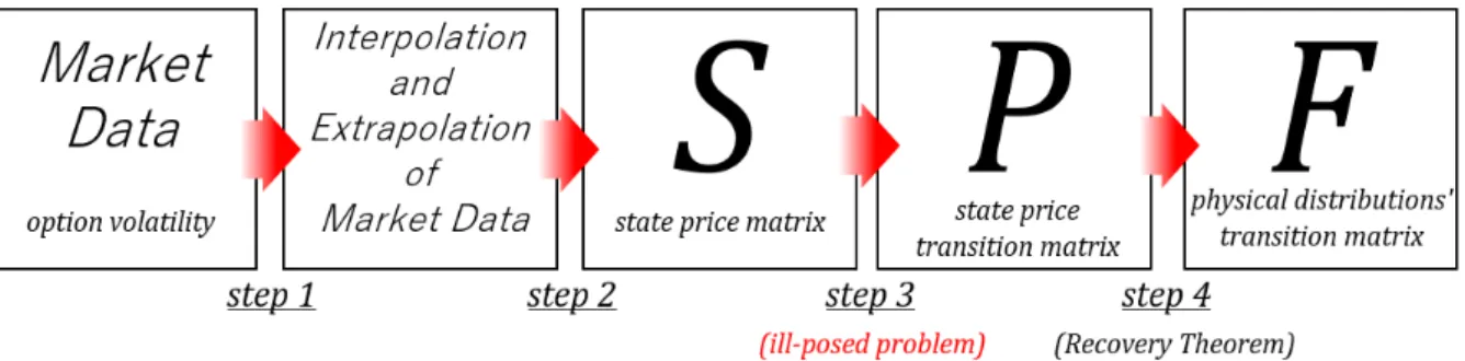
2.3 How to Apply to Empirical Data

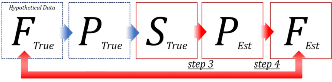
The application procedure of the theorem to the empirical data is composed by 4 steps.

Figure 2.1: Application process of the Recovery Theorem

Step 1

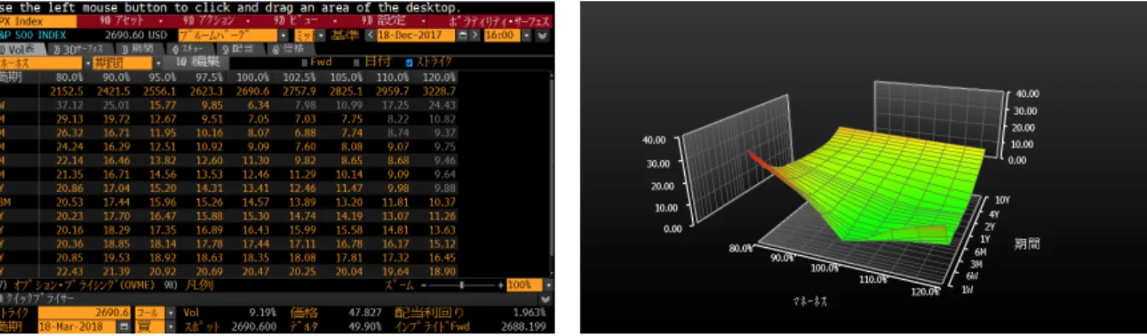
This step is about the interpolation and the extrapolation of the implied-volatility data. In the process of application, option data (i.e., implied-volatility-surface) is required to create a state price matrix S. However, not so many option implied- volatilities are observable in the market. (See Figure 2.2)

2Perron–Frobenius theorem is the theorem that guarantees following relations.

LetA= (aij) be a primitive matrix. Then there exists an eigenvaluersuch that:

(1)ris positive;

(2) the associated left and right eigenvectors can be chosen strictly positive componentwise;

(3) the eigen vectors associated withrare unique up to constant multiples;

(4)r >|λ|for any other eigenvalueλofA;

(5) ifA≥B≥0andβ is an eigenvalue ofB, then|β| ≤r. Moreover,|β|=rimpliesB=A;

(6) min_i∑

ja_ij ≤r≤max_i∑

ja_ij.

(14)

Figure 2.2: Volatility-surface for S&P500 European Option on December 18th, 2017 (Data source: Bloomberg L.P.)

To calculate the state price matrix in the next step, smooth implied-volatility- surface at each option maturity is required. We therefore interpolate the data. Also, around the deep out-of-the-money and deep in-the-money, option liquidity is so low that it is diﬃcult to use it straightforwardly as the reliable data. An extrapolation is also necessary in this step.

In the field of interpolation and extrapolation, many approaches are proposed. We introduce some literature related to them. The first is Figlewsk (2010). Figlewsk (2010) proposes the interpolation and extrapolation approach, which uses spline functions and generalized-extreme-value (GEV) functions.

Spline Interpolation

The spline interpolation is a form of interpolation that is a special type of piecewise polynomial called a spline. Spline interpolation is often preferred over polynomial interpolation because the interpolation error can be made small even when using low degree polynomials for the spline. Generally, spline is the term for elastic rulers that are bent to pass through a number of predefined points (“knot”). The approach to mathematically model the shape of such elastic rulers fixed by n+ 1 knots {(x_i, y_i) : i = 0,1,· · · , n} is to interpolate between all the pairs of knots (x_i, y_i) and (x_i+1, y_i+1) with polynomials y=S_i(x), i= 1,2,· · · , n.

As the spline will take a shape that minimizes the bending (under the constraint of passing through all knots), both y^′ and y^′′ will be continuous everywhere and at the knots. To achieve this, one must have that

S_i^′(x_i) = S_i^′₋₁(x_i) i= 1,2,· · · , n, (2.22) S_i^′′(x_i) = S_i^′′₋₁(x_i) i= 1,2,· · · , n. (2.23)

(15)

This is the case of degree 3 spline function. Though the classical approach is to use polynomials of degree 3 (i.e. cubic-spline), Figlewsk (2010) proposes degree 4 spline function to get smooth risk-neutral distribution. Figlewsk (2010) also mentions the possibility of over-fitting in the case of degree 5 or higher spline functions.

Extrapolation of the Generalized-Extreme-Value Function

There are not so much implied volatility data quoted in the market, especially deep out-of-the-money and deep in-the-money. Thus, adding tail parts to the risk-neutral distribution is a necessary step, especially when we think about risk management.

Figlewsk (2010) proposes one extrapolation approach based on GEV function. GEV function is defined as

F(x) =exp [

− {

1 +ξ

(−x−µ σ

)}₋1/ξ]

, (2.24)

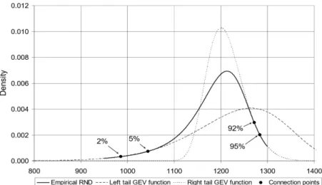
whereξis a fixed number, which is a parameter that controls the shape of the distribution, and µand σ are parameters to set location and scale of the distribution. Hence, we need to set the three GEV parameters, which means that we prepare at least three constraint conditions on the tail. We use the expressions F_{EV L}(·) and F_{EV R}(·) to denote the approximating GEV distributions for the left and right tails, respectively, withf_{EV L}(·) andf_{EV R}(·) as the corresponding density functions. F_{RN D}(·) andf_{RN D}(·) denote the estimated empirical risk-neutral distribution and its density functions, re- spectivery.

Let X(α) denote the exercise price corresponding to the α-quantile of the risk- neutral distribution. That is, F_{RN D}(X(α)) =α. First, we choose the value of αwhere the GEV tail is to begin, and then a second, more extreme point on the tail, that will be used in matching the GEV tail shape to that of the empirical risk-neutral density.

These values will be denoted by α_0R and α_1R, respectively, for the right tail and α_0L and α_1L for the left.

After setting 4 points,α_0L, α_1L andα_0R, α_1R, consider to fit a GEV tail for the risk- neutral distribution. The first condition is that the total probability in the tail must be the same for the risk-neutral distribution and the GEV approximation. Figlewsk (2010) mentions that the GEV density has the same shape as the risk-neutral distribution in the area of the tail where the two distributions overlap, thus uses the other two degrees of freedom to set the two densities equal at α0R and α1R. Namely,

(16)

Figure 2.3: Image of the risk-neutral density and fitted GEV functions (Source:

Figlewsk, S. (2010). “Estimating the implied risk neutral density for the US market portfolio.” page 41)

F_{EV R}(X(α_0R)) = α_0R, (2.25)

f_{EV R}(X(α_0R)) = f_{RN D}(X(α_0R)), (2.26) fEV R(X(α1R)) = fRN D(X(α1R)). (2.27) Similarly, constraint conditions on the left tail can be described. Then, we solve each tail’s minimization problem. The GEV parameters can be found easily by using a standard optimization procedure.

Interpolation and Extrapolation of the Double-Log-Normal Distribution The second is Bliss and Panigirtzoglou (2002). They denote double-log-normal approximating function for interpolating and extrapolating the risk-neutral density.

LetC_t(K) and P_t(K) denote the European call and put option price at timetwith strike K and option maturity T, respectively. C_t(K) and P_t(K) can be expressed by

C_t(K) = e⁻^rT

∫ +∞ K

(S_T −K)dq(S_T), (2.28) P_t(K) = e⁻^rT

∫ K

−∞

(K −S_T)dq(S_T). (2.29)

(17)

Double-log-normal function ˆL(·) is denoted by using 2 log-normal distribution L(·) as L(Sˆ _T) = θL(S_T|µ₁, σ₁, S_t) + (1−θ)L(S_T|µ₂, σ₂, S_t), θ ∈[0,1], (2.30) L(S_T) = 1

S_Tσ√

2πτexp

{−[logS_T −logS_t−(µ− ¹₂σ²)T]² 2σ²T

}

. (2.31)

In the case of the European call option, by putting (2.30) into (2.28), we get Cˆ_t(K|µ₁, σ₁, µ₂, σ₂, θ) = e⁻^rT{θ

∫ +∞ K

(S_T −K)L(S_T|µ₁, σ₁, S_t)dS_T + (1−θ)

∫ _+∞

K

(S_T −K)L(S_T|µ₂, σ₂, S_t)dS_T}. (2.32) The European put option price can be described as well. 5 parameters,{µ₁, σ₁, µ₂, σ₂, θ}, are estimated by solving the optimization problem (2.33) below, where N_c, N_p describe the number of call options and put options observed in the market. w_i, w_j are interpreted as weight for each optimization, and they are generally determined referring to each option’s liquidity.

µ1,σmin1,µ2,σ2,θ

Nc

∑

i=1

w_i[C_t(K_i)−Cˆ_t(K_i|µ₁, σ₁, µ₂, σ₂, θ)]²+

Np

∑

j=1

wj[Pt(Ki)−Pˆt(Ki|µ1, σ1, µ2, σ2, θ)]², (2.33)

s.t

Nc

∑

i=1

w_i+

Np

∑

j=1

w_j = 1, w_i, w_j ≥0.

In Bliss and Panigirtzoglou (2002), they mention 2 log-normal functions are best to interpolate and extrapolate the distribution from the view point of the stability.

Step 2

DefineS_t,(t = 1,· · ·, m) as a 1×n state price vector with option maturity t, and similarly define anm×n matrixSthat contains eachS_t,(t= 1,· · · , m). The objective of step 2 is to estimate S from implied volatility data. The most famous method is based on Breeden and Litzenberger (1978). They show that we get the state price by diﬀerentiating the option price twice with the option’s strike.³ Many other methods, e.g., Bliss and Panigirtzoglou (2002), Melic and Thomas, Ludwig (2015) and Ludwig (2015), are also proposed.

3The derivation is contained in appendix A

(18)

Step 3

In Step 3, we estimate the state price transition matrix P from S. There is no sophisticated method about estimating P, so we need to think out the estimation method. Ross (2015) estimates P by using the optimization problem as

maxP ||StP−St+1||²2, (2.34) where || · ||²2 denotes the Euclidean norm. Audrino, Huitema and Ludwig (2015) point out, in the case that the dimension ofPis not small, the optimization problem in Ross (2015) causes the ill-posed problem. The ill-posed problem is a situation that there are some candidates of optimal solutions whose objective function values are almost the same. Thus, by adding the regularization term, Audrino, Huitema and Ludwig (2015) propose a new method, known as Tikhonov method, to curve the outbreak of the ill-posed problem:

maxP ||S_tP−S_t+1||+ς||P||²₂, (2.35) where the second term is the regularization term, and ς is a regularization parameter, which controls the trade-oﬀ between the fitting and the stability of P. In other words, in this method, each element of P can not reach a high number because of the regularization term.

In the same spirit, Kiriu and Hibiki (2015), by adding another type of the regularization term, propose a new approach:

maxP ||S_tP−S_t+1||+ς||P−P¯||²2, (2.36) where the second term is the regularization term like Audrino, Huitema and Ludwig (2015). The diﬀerence between them is the existence of ¯P. Kiriu and Hibiki (2015), before solving the optimization problem, set ¯P that is expected to be similar to P.

This approach shows a more stable performance than Audrino, Huitema and Ludwig (2015).

However, this approach still has some drawbacks. First, we need to set ς and ¯P beforehand based on the historical data (i.e., backward-looking approach). In addition, how to set plausible ¯P is a quite diﬃcult problem, and also the result fluctuates according to the level of ς.

There are other approaches proposed in the literature. For example, Fabio, Julian and Yang (2016) try to prevent the ill-posed problem by adding 6 constraint conditions including the single-peak-property. Morikawa (2016) solves the ill-posed problem by using the optimization problem with only the constraint condition of the single-peak property.

(19)

Step 4

Step 4 is straightforward. By using P, simply apply the Recovery Theorem to recover a unique physical transition matrix F.

2.4 Literature Review of the Recovery Theorem

The year when Steve Ross first released the theorem was 2011, though the year when the theorem was accepted by the Journal of Finance was 2015. After the first appearance, many researchers have been analyzing this theorem and trying to apply it to the empirical data.

There are 3 types of studies related to the Recovery Theorem. The first is the research how to solve the ill-posed problem as we have already mentioned.

The second is the numerical test by using the theorem. Ross (2015) applies it to S&P 500 to recover the physical distribution and compares it with the historical distribution.

After that, Martin and Ross (2013) denote how to recover the interest rate distribution of the long-term government bond. Audrino, Huitema and Ludwig (2015) show S&P 500 physical distribution and calculate the diﬀerence between physical distributions and risk-neutral distributions (i.e., moment-risk-premium). Jensen, Lando and Pedersen (2015), by using S&P 500, research about the regression analysis for the distribution’s expected return and the volatility under the physical measure.

The third is the expansion of the theorem. In the Recovery Theorem, discrete time and a finite number of states are assumed. Carr and Yu (2012) and Dubynskiy and Goldstein (2013) show the availability of application of the theorem under the continuous time assumption. In addition, Walden (2014) and Park (2014) propose the new theorem without the assumption of finite states. Also, Jensen, Lando and Pedersen (2015) point out that the assumption of the pricing kernel in Ross (2015) is not realistic intuitively and propose a new theorem without the assumption by introducing the term structure of the discount factor.

(20)

Chapter 3 The Tree Approach

Audrino, Huitema and Ludwig (2014), and Kiriu and Hibiki (2015) provide us stable state price transition matrix P. However, as we mentioned, it is quite diﬃcult to explain the theoretical background of the regularization term. Moreover, these approaches use the historical data.

Fabio, Julian and Yang (2016) and Morikawa (2016) add some constraint condition to increase the stability. It decreases the degree of freedom of the optimization problem, their approaches therefore may archive stable result under the normal environment.

However, it may not be able to fit the emergent situation such as the global financial crisis. This is the situation what risk managers really want to predict beforehand.

In this chapter, we propose a new approach, which is more stable and straightforward, and show the high accuracy of the recover and fast computational time.

3.1 Trinomial Tree Approach

3.1.1 Concept of the Approach

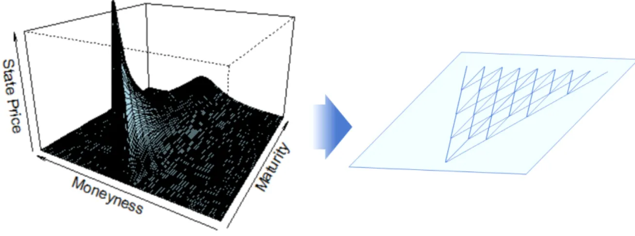
First, we describe the state price matrix for S&P 500 induced from the European option data to get the image that what type of a transition matrix is likely fitted to the data. In Figure 3.1 is the state price of the European option of S&P 500 on October 10th, 2010.

It describes that the state price is gradually diﬀusing as the option maturity goes on. Therefore, it seems possible to depict its transition matrix Pby the tree structure.

We name it “tree approach”.

(21)

Figure 3.1: State price for S&P500 on October 10th, 2010 and trinomial tree structure Theoretical background

We check the theoretical consistency of the tree approach. As the tree approach is an approximation method of describing a diﬀusion process, we confirm that the state price follows a stochastic diﬀerential equation.

LetS(t) denote an asset price at time t and B(t) denote a bank-saving-account at time t, and assume that they follow stochastic diﬀerential equations as follows:

dS(t)

S(t) = µ(t)dt+σ(t)dz(t), (3.1)

dB(t)

B(t) = r(t)dt. (3.2)

Under the assumption of arbitrage-free and complete market,¹ let us define the exponential martingale as

Y(t) =e^θz(t)⁻^θ²^t/2. (3.3)

1The fundamental theorems of asset pricing provides necessary and suﬃcient conditions for a market to be arbitrage-free and for a market to be complete. In a discrete market, the following hold:

1. A discrete market, on a discrete probability space (Ω,F,P), is arbitrage free if, and only if, there exists at least one risk-neutral probability measure that is equivalent to the original probability measureP (The First Fundamental Theorem of Asset Pricing).

2. An arbitrage free market (S, B) consisting of a collection of stocksS and a risk-free bondB is complete if and only if there exists a unique risk-neutral measure that is equivalent toP and has numeraireB (The Second Fundamental Theorem of Asset Pricing).

(22)

The above equation satisfies the following relation.

Q(A) =E^P[1_AY(t)], (3.4)

where Q denotes the risk-neutral probability. From (3.3), Y(t) can be described as dlogY(t) =θ(t)dz(t)− 1

2θ²(t)dt. (3.5)

Therefore,

dlog

(Y(t) B(t)

)

= (

−1

2θ²(t)−r(t) )

dt+θ(t)dz(t). (3.6) Since the state price density ϕ is described as ^Y_B(t)^(t), and under the arbitrage-free and complete market assumption, ϕ exists uniquely. Moreover, from Ito’s lemma,ϕ is expressed as follows:

dϕ(t)

ϕ(t) =−r(t)dt+θ(t)dz(t). (3.7)

Then, ϕ(t) and the state price p(t) can be expressed as below:

ϕ(t) = 1 e^r(t)t

dQ(t)

dP(t), (3.8)

p(t) = ϕ(t)dP(t). (3.9)

We already showed that ϕ(t) can be described by a stochastic differential equation (i.e., diffusion process). So, if we assume dPfollows a diffusion process, state price p(t) also can be written as a diffusion process. Hence, it is natural to describe the state price transition matrix P by the tree structure.

Optimization Problem under the Approach

We can formulate the optimization problem under the tree approach as follows:

minP T−1

∑

t=1

||S_tP^k−S_t+1||²₂, k ≥1, (3.10) wherePis a tri-diagonal matrix andkis a natural number, which controls the diﬀusion speed of the state price. It is much simpler than other approaches.

(23)

3.1.2 Numerical Test

We investigate the accuracy of the recovery under the tree approach by some numerical tests.

Procedure of Numerical Test

Figure 3.2 represents the framework of the test. We refer the method in Kiriu and Hibiki (2015).

Figure 3.2: Procedure of the numerical test

1. Set the two simulated matrices; physical transition matrix F_{T rue} and pricing kernel Φ_{T rue}.

2. Calculate the true state price transition matrix P_{T rue} and true state price S_{T rue} in backward order.

3. Estimate P_Est from S_{T rue} by using Step 3 of the Recovery Theorem. S_{T rue} is composed by a large number of state price vector St,T rue. In this step, we use 12 state price vectors (S_{T ure} = (S_{1,T rue},· · · ,S_{12,T rue})^T)

4. Similarly, Apply Step 4 of the theorem to recover F_Est Next, we describe the setting in more detail.

Physical Transition Matrix

The physical probability transition matrix FT rue is a 13 × 13 matrix and it is discretely described by every 4%. So, this matrix is equally divided from -30% to 30%.

Also, S&P 500 historical data (from January 3rd, 1950 to January 3rd, 2014) are used

(24)

to generate F_{T rue} because of the high liquidly and long data availability.

First, we set a reference date and calculate a 30-calendar-days return from the reference date. We use the day before a holiday in the case of a holiday. After counting the number of state transitions in each period, we sum up each element of the matrix.

Finally, we divide each of them by each sum of the row elements to make a probability transition matrix.

Pricing Kernel

In the Recovery Theorem, we suppose that the pricing kernel is described by ϕ(θt+1|θt) = δh(θt+1)

h(θ_t) . (3.11)

As we explained,h(θt) is interpreted as the derivative, type of an investor’s utility.

In addition, we suppose that h(θ_t) is written as derivative of the constant relative risk aversion (CRRA) function U(θ_i) = θ_i^1−γ^R/(1−γ_R), where γ_R is the relative risk aversion. Ifθi can be described by using the rate of returnri, we can therefore calculate the pricing kernel as

p^{T rue}_i,j = δU^′(θ_j)

U^′(θ_i)f_i,j^{T rue} (3.12)

= δθ⁻_j^γ^R

θ⁻_i ^γ^Rf_i,j^{T rue} (3.13)

= δ

(1 +r_j 1 +r_i

)₋γR

f_i,j^{T rue}. (3.14)

We therefore can calculate PT rue from (3.14). In this test, γR = 3, and δ = 0.999 are used.

Evaluation Criteria of the Estimation Accuracy

We use Kullback–Leibler divergence (KL divergence) as the evaluation criteria. Let us define F_i^{T rue} as the probability under the physical measure in the θ_i, and similarly define F_iÊst as well. After recovering FÊst, compare FÊst and F^{T rue} as follows:

D_KL(F^Est|F^{T rue}) :=

∑n i=1

F_i^Estln

( F_i^Est F_i^{T rue}

)

. (3.15)

When the estimated distribution is exactly equal to the true distribution, D_KL is equal to zero.

(25)

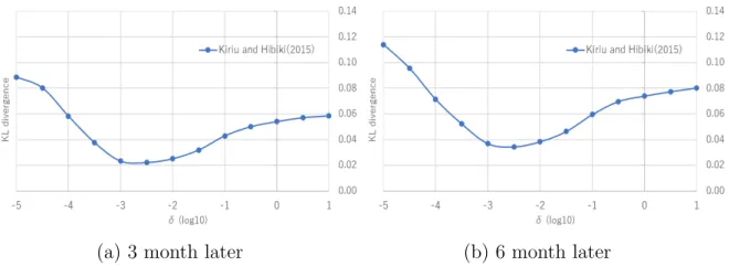
Result

First, we compare Kiriu and Hibiki (2015) approach withς (ς=10⁻⁵,· · · ,10¹). Fig- ure 3.3 shows the KL divergence of 3 month later and 6 month later. Aroundς = 10⁻^2.5, this approach attain the lowest KL divergence. However, the result fluctuates a lot when the level of ς moves.

(a) 3 month later (b) 6 month later

Figure 3.3: KL divergence of the recovered physical distribution in the case of Kiriu and Hibiki (2015)

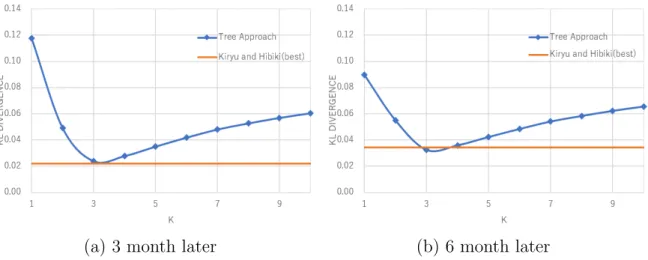
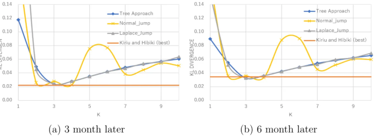
Next, Figure 3.4 shows the KL divergence in the case of the tree approach with k (k = 1,· · · ,10). ² The tree approach of both 3 month and 6 month later attains the lowest KL divergence in the case of k= 3. In addition, the result of the tree approach is as low as or a little bit better than best result of Kiriu and Hibiki (2015).

Same as Kirui and Hibiki (2015), parameter k influences the KL divergence. How- ever, P is a tri-diagonal matrix in the tree approach. So, it is natural why the case of k = 1 marks the higher KL divergence. Therefore, k = 1 is generally never chosen.

In addition, the cases of the higher k,k = 6,· · · ,10 , are almost meaningless, because P is a 13×13 tri-diagonal matrix. Therefore, in the case of k = 5, most elements in the matrix have positive number. For example, we show the P with k = 2 as below.

Nearly 50% of the elements are covered even in the case of k = 2.

2In this analysis, we use a 13×13 matrix. So, higherkis not required. However, we are checking the higher case to see its behavior.

(26)

Figure 3.4: KL divergence of the recovered distribution under the tree approach

P² =







0.63 0.17 0.17 0.03 0.0 0.0 0.0 0.0 0.0 0.0 0.0 0.0 0.0 0.29 0.14 0.36 0.18 0.03 0.0 0.0 0.0 0.0 0.0 0.0 0.0 0.0 0.11 0.13 0.37 0.29 0.08 0.01 0.0 0.0 0.0 0.0 0.0 0.0 0.0 0.01 0.05 0.21 0.39 0.27 0.07 0.001 0.0 0.0 0.0 0.0 0.0 0.0 0.0 0.01 0.04 0.19 0.42 0.27 0.07 0.01 0.0 0.0 0.0 0.0 0.0 0.0 0.0 0.00 0.03 0.18 0.42 0.28 0.07 0.01 0.0 0.0 0.0 0.0 0.0 0.0 0.0 0.00 0.03 0.18 0.43 0.29 0.06 0.00 0.0 0.0 0.0 0.0 0.0 0.0 0.0 0.00 0.03 0.18 0.46 0.26 0.06 0.00 0.0 0.0 0.0 0.0 0.0 0.0 0.0 0.00 0.03 0.17 0.47 0.27 0.06 0.00 0.0 0.0 0.0 0.0 0.0 0.0 0.0 0.00 0.02 0.15 0.47 0.29 0.7 0.01 0.0 0.0 0.0 0.0 0.0 0.0 0.0 0.00 0.02 0.16 0.46 0.29 0.7 0.0 0.0 0.0 0.0 0.0 0.0 0.0 0.0 0.00 0.02 0.19 0.45 0.34 0.0 0.0 0.0 0.0 0.0 0.0 0.0 0.0 0.0 0.00 0.02 0.17 0.81







(3.16) Moreover, it is understandable why the KL divergence increases as k increases. It

seems very diﬃcult to solve the optimization problem when k is higher, because the optimization problem becomes more complected.

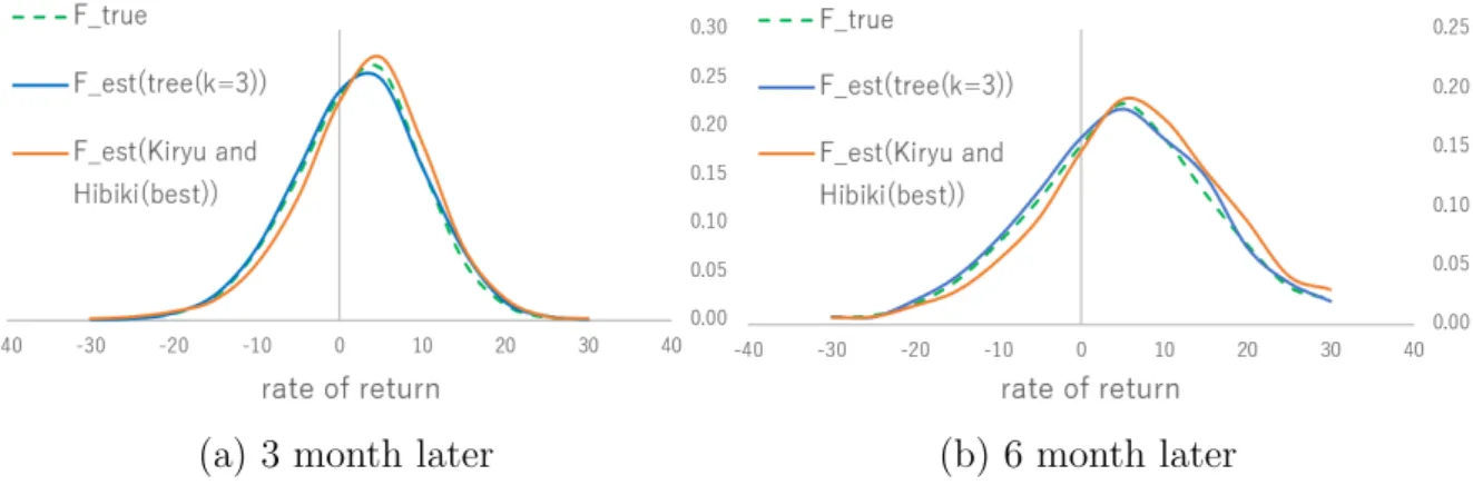
Figure 3.5 shows recovered physical distributions of 3 month later and 6 month later. The new approach is more fitted to true physical distributions too.

(27)

Figure 3.5: Recovered distribution under tree approach

3.1.3 Characteristics of the Approach

We summarize the characteristics of the tree approach as bellow:

• < Robust theoretical background and not depending on historical data>

In the case of Kiriu and Hibiki (2015), finding the suitable δ beforehand seems diﬃcult and its theoretical background is very weak. However, the tree approach is correct that the state price transition can be depicted as a diﬀusion process, and it is consistent with finance theory. Furthermore, this approach is much stable with any k. Therefore, historical data is not needed at all.

• < Stable recovery >

The recovery accuracy in the tree approach is better than Kiriu and Hibiki (2015).

• < Fast computational time of the recovery >

The Recovery Theorem has been expected to apply to not only risk management, but also investment strategies. Therefore, computational time is a significant issue. As the elements that we have to estimate are much fewer in the tree approach, the recovery speed is faster. Actually, it takes only around 6.73 seconds to recover the 1 physical distribution in the tree approach. However, Kiriu and Hibiki (2015) need 19.60 seconds.

3.2 Tree Approach with Jumps

P^k induced from the tree approach is a multi-diagonal matrix. Except for upper and lower rows, each row has the same number of positive elements. So, if k is lower,

(28)

this approach can not catch the radical state price movement. In the tree approach, however, the KL divergence fluctuation is observable if higherk is used. In this section, in order to catch such radical state price movements, we consider adding the jump process to the tree approach. The processes described below are popular jump process, where J is a random variable, h is a fixed parameter, which satisfies h= E[J −1], A is an arbitrary financial instrument, which has driftµ_A and volatilityσ_A. Also, N_tis a Poisson process with intensityλ. z_t, N_t andJ are generally supposed to be respectively independent.

• Normal jump diﬀusion process dA(t)

A(t−) = (µA−λh)dt+σAdzt+ (J−1)dNt, J ∼Φ(µ, σ²). (3.17)

• Lognormal jump diﬀusion process (Merton model) dA(t)

A(t−) = (µ_A−λh)dt+σ_Adz_t+ (J−1)dN_t, lnJ ∼Φ(µ, σ²). (3.18)

• Laplacian jump diﬀusion process (Kou model) dA(t)

A(t−) = (µ_A−λh)dt+σ_Adz_t+ (J −1)dN_t. (3.19) In the Kou model, the probability density function of lnJ is described as below.

1l is an indicator function.

pη₁e⁻^η¹^y1l_{_y_≥₀_}+ (1−p)η₁e⁻^η²^y1l_{_y<0_}, η₁ >1, η₂ >0. (3.20) Discrete compound Poisson distributions can be also implemented in the tree approach. However, we need to set each jump width beforehand. It means that it increases a chance of the using discretion. In addition, increasing the number of parameters eliminates the tree approach characteristics. Thus, in this thesis, we treat only continuous jump models.

3.2.1 Implementation Method

Same as the tree approach, the following optimization problem is used in the tree model with jumps:

minP n−1

∑

t=1

||S_tP^k−S_t+1||²₂. (3.21)

(29)

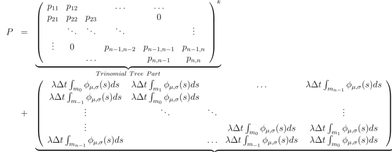
In the tree approach, we assume thatP is a tri-diagonal matrix. However, to take the jump process into account, we add a jump term in P. For example,P in the tree approach with normal jump process is described as

P =







p11 p12 . . . . . .

p₂₁ p₂₂ p₂₃ 0

. .. ... . .. ...

... 0 pn−1,n−2 pn−1,n−1 pn−1,n

. . . p_n,n₋₁ p_n,n







k

| {z }

T rinomial T ree P art

+







λ∆t∫

m0ϕ_µ,σ(s)ds λ∆t∫

m1ϕ_µ,σ(s)ds . . . λ∆t∫

mn−1ϕ_µ,σ(s)ds λ∆t∫

m₋₁ϕ_µ,σ(s)ds λ∆t∫

m0ϕ_µ,σ(s)ds

... . .. . .. ...

... λ∆t∫

m_n−1ϕ_µ,σ(s)ds . . . λ∆t∫

m₋₁ϕ_µ,σ(s)ds λ∆t∫

m0ϕ_µ,σ(s)ds







| {z }

J ump P art

,

(3.22) where ϕ_µ,σ(s) is a normal probability density function with mean µ and deviation σ,

and m_i is the range.

3.2.2 Numerical Test

We compare the KL divergence between the tree approach with jumps and the simple tree approach. Only normal model and the Kou model are used in this test.

The method of this numerical test is the same as the method mentioned in 3.1.

Result

Figure 3.6 shows that the KL divergence with k of 3 months later and 6 months later, respectively. The KL divergences are as same as or worse than the simple tree approach. In addition, the result of the tree approach with normal jumps is fluctuated when k is higher. In the tree approach with jumps, the number of parameters is larger than the simple tree approach. Because of that, the optimization problem is more complicated and it might cause this fluctuation.

Under the tree approach with lowerk, P^k can not describe the high volatility. So, atk= 2 or 3, the KL divergence of jump approaches are a little bit better than the tree

(30)

Figure 3.6: KL divergence in the tree approach with jump

approach. But, in the case of the tree approach with higherk,P^k can access to almost all states. So the diﬀerence between the tree approach and the tree approach with jumps is diminished. It might be useful to add a jump process to the tree approach when big matrix P is used. However, this result shows, in the case of smaller matrix such as 13×13, the merit of adding jump process is limited.

3.3 Non-Stationary Tree Approach

3.3.1 Drawback of the Tree Approach

As Figure 3.1 shows, the state price spreads to the left and right over the option maturity. Suppose that a state price with the option maturity t satisfies

dS(t) = µdt+σdz (3.23)

Then its volatility satisfies

E[{S(T)−E[S(T)]}²] = σ²T. (3.24) Since each historical volatility can be calculated by using (3.24), we can create a daily single linear regression model for the volatility with the option maturity to get to know about the propensity of the volatility of the state price. Figure 3.7 describes the daily coeﬃcients of the single regression models.

(31)

Figure 3.7: Coeﬃcient of S&P500’s single regression model (from October 20th, 2010 to June 1st, 2017)

Option maturity Variance Volatility

1 month 1.441 4.992

2 month 1.979 4.848

3 month 2.461 4.923

6 month 3.590 5.077

12 month 5.331 5.331

18 month 6.744 5.507

24 month 7.999 5.656

Table 3.1: Average state price volatility with the option maturity (from October 20th, 2010 to June 1st, 2017)

If coeﬃcients are around 0, it means that the volatility is not fluctuated with the option maturity. Thus, we can assume that the volatility is a fixed number. However, coeﬃcients of the historical data are actually fluctuated, and most of them attain positive numbers. In the tree approach, same P is used to all option maturities (i.e.

stationary approach). Hence, we consider the non-stationary tree approach to grasp this propensity.

3.3.2 Implementation Method

To grasp the non-stationarity, we propose 2 methods.

1. Double tree approach

This approach uses 2 state price matrices,P^′andP^′′, induced from 2 optimization

(32)

problems. P^′ denotes the transition matrix which priorities the first half of the data. P^′′, on the other hand, is estimated with mainly the later half of the data.

This procedure has 2 steps.

(a) EstimateP_t by solving the optimization problems P^′ and P^′′:

P_t = q_tP^′^k + (1−q_t)P^′′^k 0≤q_t ≤1, (3.25) min

P^′ n−1

∑

t=1

ω_t^′||S_tP^′^k −S_t+1||²2, (3.26)

minP^′′

n−1

∑

t=1

ω_t^′′||StP^′′^k−St+1||²2, (3.27) where ω_t^′, ω_t^′′ are coeﬃcient numbers calculated by functions such as power functions,ω_t^′ =a^1−t, ω^′′_t =a^t.

(b) Determine the optimalq_t in (3.25) by solving the optimization problem minqt

∑n−1 t=1

||S_tP_t−S_t+1||²2. (3.28) 2. Tree approach with the option maturityt

This approach prepares P_t to each option maturity t. ω_t denotes a distribution like Laplacian distribution. After choosing the distribution, estimate Pt with each option maturity. Namely,

minPt

n−1

∑

t=1

ωt||StPt−St+1||. (3.29)

3.3.3 Numerical Test

Procedure of Numerical Test

The basic procedure is the same as the numerical test in the tree approach. First, prepare the true physical transition matrix and the pricing kernel. Second, calculate the state price transition matrix and the state price. Finally, estimate the physical transition matrix by using the Recovery Theorem. All of the same parameters are basically used in this analysis. However, under the non-stationary assumption, in order to get more stable results, we use 48 state price vectors (S_{T rue} = (S_{1,T rue},· · · ,S_{48,T rue})^T).

Also, we use non-stationary F_{t,T rue} with each option maturity t instead of F_{T rue}. Fig- ure 3.8 shows the image of the procedure in the case of the double tree approach.