Reeb components of leafwise complex foliations and their symmetries

(1)

Reeb components of leafwise complex foliations and their symmetries

Tomohiro HORIUCHI

Department of Mathematics

Graduate School of Science and Engineering Chuo University

March 2016

(2)

Chapter 1 Introduction

In this thesis, we study Reeb components with leafwise complex structure, focusing especially on the symmetries of the real 3 and 5-dimensional cases.

Recall that a (p+ 1)-dimensional Reeb component is a compact manifold R =D^p×S¹ with a (smooth) foliation of codimension one, whose leaves are

∂R =S^p⁻¹×S¹ and the graphs of f +c (c ∈ R), where f : intD^p → R is a smooth function such that lim_z_→_∂D^pf(z) = +∞. Here we identify R with D^p ×R/Z.

Foliations of codimension one with complex analytic leaves are drawing attentions in several complex variables because it appears as the Levi foliations of Levi flat real hypersurfaces in complex manifolds. In general, a real codimension one hypersurface M in a q-dimensional complex manifold (Y, J_Y) is said to be Levi-flat if it is locally Stein or the codimension one dis- tribution ξ =T M ∩J_Y(T M) is integrable. Namely, M is smoothly foliated by immersed complex manifolds of dimension q−1. A simple construction of Hopf manifolds admits a Levi-flat hypersurface, whose Levi foliation consists of two Reeb components. This construction is generalized in Nemirovskii’s examples [Ne] (see Chapter 6 for the details). They have non-trivial linear holonomy along toral leaves. On the other hand, Reeb components with flat holonomy appears in turbulization or in Dehn surgery (see Chapter 2 for the details). In this thesis, we consider Reeb components with holonomy tangent to the identity to the m-th (0≤m≤ ∞) order at the boundaries.

In Chapter 4, we study the group of all leafwise holomorphic automorphisms of 3-dimensional Reeb components with leafwise complex foliations.

In particular, in the case where the Reeb component is obtained by the Hopf construction, we determine the structure of the group. Main theorem is the following.

Main Theorem 1 Let R be a 3-dimensional leafwise complex Reeb component obtained by Hopf construction and φ∈Diﬀ^∞([0,∞)) the holonomy tangent to them-th (0≤m≤ ∞) order at the boundary elliptic curveH. In particular, the modulus of H is _2πi⁻¹ logλ, where λ is a complex number such that |λ|>1. Then the group AutR of leafwise holomorphic automorphisms

(4)

of R is isomorphic to the semi-direct product (K⋊Z_φ)⋊Aut₀H

where Aut₀H is the identity component of the automorphism group of H, Z_φ is the centralizer of φ in Diﬀ^∞([0,∞)) and K is the space of smooth C-valued functions β on [0,∞) satisfying the equation

(I) : β(φ(x)) = λβ(x), β ∈C^∞([0,∞);C).

The space K of solutions to the equation (I) on [0,∞) depends on the tangency ofφ. Ifm= 0, i.e.,φis not tangent to the idnetiy,Kis isomorphic to C or {0}. If m > 0, i.e., φ is tangent to the identity, K coincides with the space Zφ,λ of solutions to (I) on (0,∞). In particular, K is an infinite dimensional vector space. The proof of above claims is in Chapter 3. Key points of the proof are the (in)finitely tangency of φ, the formula of Fa´a di Bruno, Sternberg’s linearlization [St], Takens’ normal forms [Ta], and a classical theory on Fourier expansion of smooth periodic functions.

The centralizer Z_φ in Diff^∞([0,∞)) is known to be fairly wild. Let Z_φ^r be the centralizer of φ in Diff^r([0,∞)) (1 ≤ r ≤ ∞). Then Z_φ^r contains the infinite cyclic subgroup generated by φ. Moreover, in the case of r= 1, theorems by Szekeres [Sz] and Kopell [Kop] show that Z_φ¹ is a one-parameter subgroup of Diff¹([0,∞)). For r≥2, we obtain the following inclusions.

Z∼={φⁿ; n ∈Z} ⊂ Z_φ^r ⊂ Z_φ¹ ∼=R

According to theorems by Sternberg and Takens, ifφis not infinitely tangent to the identity at the origin, then Z_φ =Z_φ^∞is isomorphic toR. On the other hand, Sergeraert [Se] constructed a diﬀeomorphism φwhose centralizerZ_φ² is strictly contained in R and Eynard [Ey] constructed φsuch that Z_φ^r (r ≥2) is a proper, dense and uncountable subgroup of R.

In the case of complex leaf dimension 2, the boundary leaf of a Reeb component is called a primary Hopf surface. Kodaira [Ko1] classified the primary Hopf surfaces into five types and gave normal form in each case (Theorem 5.1). In Chapter 5, we compute the group of leafwise holomorphic automorphisms of 5-dimensional leafwise complex Reeb components with holonomy infinitely tangent to the identity for each type of the boundary Hopf surface relying on the normal form and obtain the following.

Main Theorem 2 LetRbe a 5-dimensional leafwise complex Reeb component obtained by the Hopf construction andφ∈Diﬀ^∞([0,∞)) the holonomy tangent to the identity to them-th (1≤m ≤ ∞) order at the boundary Hopf surface H. Then AutR admits a following sequence of extensions.

(5)

1 → Aut(R, H) → AutR → AutH →1, 0→ K → Aut(R, H) → Z_φ →1

where AutH is the automorphism group of H, Aut(R, H) is the kernel of the restriction map from AutR to AutH and K is an infinite dimensional vector space depending on the normal form ofH (see Theorem 5.9 and 5.11).

Acknowledgements The author would like to express my gratitude and respect to Professor Yoshihiko Mitsumatsu. This thesis could not be com- pleted without his advice and support.

The author would like to thank Professors Youichi Miyaoka, Sigeaki Miyoshi and Tatsuru Takakura for their advice and consideration.

The author is very grateful to the members of Saturday Seminar (a.k.a Dosemi) at the Tokyo Insitute of Technology, especially to Kazuo Masuda, Takashi Inaba, Atsushi Sato, Noboru Ogawa and Masanori Adachi for their valuable comments and suggestions.

Finally, the author would like to thank all Professors and staﬀs of De- partment of Mathematics for their consideration and support.

(6)

Chapter 2 Preliminaries

2.1 Leafwise complex structure

Let M be a (2n+q)-dimensional smooth manifold, F a smooth foliation of codimension q on M and p = 2n the dimension of leaves. We refer general basics for foliation theory to [CC].

Definition 2.1(Leafwise complex structure, cf. [MV]) (M,F) is said to be equipped with a leafwise complex structure if (M,F) is given by a foliation atlas {(U_α, ϕ_α)} such thatϕ_α(U_α) is an open set of Cⁿ×R^q and that in each coordinate change

ϕ_α(U_α∩U_β)∋(z, x)7→ϕ_β◦ϕ⁻_α¹(z, x) = (w_αβ(z, x), y_αβ(x))∈ϕ_β(U_α∩U_β) w_αβ is holomorphic with respect to z.

This definition is equivalent to that the foliation has complex structures varying smoothly in transverse directions,i.e., the tangent bundleτF to the foliation F is equipped with a smooth integrable almost complex structure J. We call (M,F, J) a leafwise complex foliation.

Definition 2.2 (Leafwise holomorphic automorphism) Let (M,F, J) be a smooth foliated manifold with leafwise complex structure. A diﬀeomorphism f : M → M is said to be a leafwise holomorphic smooth automorphism if and only if it preserves the foliation and give rise to biholomorphic maps between leaves. We denote by Aut(M,F, J), or AutM for short, the group of leafwise holomorphic smooth automorphisms of (M,F, J).

In this thesis we are only concerned with foliations of codimension one. In particular, our interest will be focused on Reeb components, especially of real dimension 3 and 5, namely in the case of n = 1 and q = 1. As we see from the examples of Nemirovskii [Ne] even a real analytic Levi-flat hypersurface in a complex manifold can admit Reeb components in its Levi foliation. In

(7)

such a case, the holonomy along the toral boundary leaf can not be tangent to the identity to the infinite order.

Apart from Levi-flats, for example, if we perform a turbulization we easily find various leafwise complex foliations admitting Reeb components with holonomy infinitely tangent to the identity.

2.2 Reeb components with complex leaves

In this section we review a particular construction of Reeb component with complex leaves and a process of turbulization which produces a new Reeb component in a leafwise complex foliation.

In order to make pasting construction easier, we introduce the following notions. Let (R,F, J) (or R for short) be a Reeb component with leafwise complex structure of complex leaf dimension n and (H, J_H) be its boundary leaf.

Definition 2.3 The Reeb component R has a tame boundary (or ‘R is tame at boundary’ for short, or even shorter ‘R is tame’) with respect to a product coordinate H ×[0, ε) of a collar neighborhood of H if it gives rise to a smooth foliation with leafwise complex structure when it is pasted with the product foliation (H×(−ε,0],{H × {x}; x ∈ (−ε,0]}, JH) along their boundary. Here each leaf H × {x} has the same complex structure as H when identified with the natural projection. Namely, the Reeb component is extended to the outside as a product foliation.

The notion of tameness was introduced in [MV].

Remark 2.4 If we forget the leafwise complex structure and consider the same notion only as foliation of codimension one, it does not depend on the choice of product coordinates on the positive side the tameness implies exactly that the holonomy is tangent to the identity to the infinite order. This is because the set of expanding diﬀeomorphisms of the half line [0,∞) which are infinitely tangent to the identity is an open convex cone and invariant under conjugation by any diﬀeomorphism. Also remark that the tameness depends only on the smooth projection of the collar neighborhood to the boundary, which the product coordinate defines. If two projections have the same infinite jets on the boundary, the tameness notion coincides for the two.

Definition 2.5 The leafwise complex structure of a Reeb component R is simple around boundary (or R has a simple complex structures around boundary) if the boundary has a collar neighborhood U ∼= H ×[0, ε) such that the restriction of the projection U =H×[0, ε) →H to each leaf in U is holomorphic

This notion should also be understood relative to the projection from a

(8)

collar neighborhood to the boundary.

The notations of tameness and simpleness apply not only to Reeb components but also to more general leafwise complex foliations of codimension one with a compact leaf or a boundary leaf.

Clearly if a Reeb component has simple complex structures around the boundary and the holonomy of the boundary leaf is infinitely tangent to the identity, it is tame with respect to the appropriate projection. The tameness condition prohibits unexpected wild behavior around boundary. In particular, in the case of complex leaf dimension = 1, it induces a strong consequence due to Meersseman and Verjovsky.

2.2.1 Reeb component by Hopf construction

Let us present a particular construction of a Reeb component with leafwise complex structure which is tame. If we remove the flat condition on the holonomy, it gives rise to more general Reeb components. These constructions are a kind of folklore.

Construction 2.6 (Hopf construction) Let φ ∈ Diff^∞([0,∞)) a diffeomorphism of the half line satisfying φ(x)−x > 0 for x > 0, namely the origin is the unique expanding fixed point. Also take a (local) biholomorphic diffeomorphism G ∈ Diff^hol(Cⁿ, O) which is expanding. This implies that for some small neighborhood D of the origin O with smooth boundary G(intD) ⊃ D and lim

k→−∞G^k(D) = {O}. Now take U = ∪^∞k=1G^k(D) ⊂ Cⁿ. Then on ˜R =U ×[0,∞)\ {(O,0)} ⊂ Cⁿ×R, take the restriction ˜F of the product foliation {Cⁿ× {x}} together with the natural complex structure on the leaves and a diﬀeomorphism T = G×φ on U ×[0,∞)\ {(O,0)}. Practically we take fairy simple diﬀeomorphisms such as linear maps asGso that U becomes the whole Cⁿ. Then on the quotient R = ˜R/T^Z a foliation F with leafwise complex structure is induced.

From the construction, it is simple around the boundary. If the holonomy is infinitely tangent to the identity it is also tame with respect to the coordinate in the construction.

The boundary U \ {O}/G^Z is a complex manifold which is a so called Hopf manifold. In the case n = 1 it is an elliptic curve and the construction is equivalent to the one with linear map as G.

Theorem 2.7 (Meersseman-Verjovsky, [MV]) Any tame Reeb component with complex leaves of complex dimension 1 is isomorphic to one of those given by the Hopf construction.

We present a couple extensions (variants) of the above construction.

(9)

Construction 2.8 Let us take the product not with the half line but with whole real line R. Let M and Φ∈Diﬀ^∞₊(R) be as follows.

• M = (U ×R\ {(O,0)})/T^′^Z, T^′ =G×Φ,

• x= 0 is an expanding unique fixed point of Φ.

M consists of two Reeb components and in exactly the same way as above a foliation with leafwise complex structure is induced on M.

Note that in this and above construction, the holonomy of the toral leaf is given by φand Φ. In these constructions, we can choose them so as to be tangent to the identity at the origin to the infinite order.

Construction 2.9 Let us take Φ as a simple linear expansion in order to extend it to a biholomorphic expansion ˜Φ∈ C. Note thatR is an invariant subspace. Fix the expansion ratio µ >1 and take the followings;

W = (U×C \ {(O,0)})/T^′′Z, T^′′ =G×Φ,˜ Φ(z) =˜ µz (z ∈C), M = (U×R \ {(O,0)})/T^′Z, T^′ =G×Φ, Φ(x) =µx (x∈R).

W is an (n + 1)-dimensional Hopf manifold, M is its Levi-flat real hypersurface with Levi foliation consisting of two Reeb components, and a unique compact leaf is the Hopf manifold (U \ {O})/G^Z of dim_C =n.

Problem 2.10 The above result by Meersseman and Verjovsky poses the following questions. We assume that the complex dimension of the leaves is one. If two Reeb components with leafwise complex structures have the same boundary holonomy and their boundary leaves are biholomorphic to each other, are they isomorphic as leafwise complex foliations? Does there exist a Reeb component with complex leaves which is not isomorphic to a tame one but with holonomy infinitely tangent to the identity? Or does there exist one which is not isomorphic to any of those given by the Hopf construction? The second form of question seems not diﬃcult to have negative answers. Anyway, those questions are asking what should be the complete invariants to determine Reeb components without assuming the tameness.

Construction 2.11 We introduce one more construction, which is pre- pared for turbuliazation. Take ˜M = (Cⁿ×R)\({O} ×R_≤0) and restrict the product action ˆT =G×Ψ to ˜M, where Ψ is an orientation preserving diffeomorphism of Rwhich fixes 0, expanding onR_≥0 = [0,∞), and contracting on the negative side R≤0 = (−∞,0], i.e. Ψ(x) > x for x < 0. On ˜M we take (the restriction of) the horizontal foliation ˜F. Then take the quotient (M,F, J_F) = ( ˜M ,F˜, J_std)/Tˆ^Z.

The non-negative part is nothing but the Reeb component constructed in 2.6 regardingφ= Ψ|R≥0. The non-positive side (N,G) = (M,F)|x≤0 remains non-compact and is in fact a foliated R_≤0-bundle with holonomy ψ = Ψ|_R_≤0. If we remove the boundary compact leaf {x = 0} from the non-positive side (N,G), it is isomorphic to (Cⁿ\ {O})×S¹. For a better description of

(10)

turbulization process, we let this identification more precise. This is done by embedding ˆT in a 1-parameter family. Take a smooth curve G_t in GL(2;C) and also a smooth curve ψt in Diﬀ^∞(R≤0) which is always tangent to the identity to the infinite order at x= 0, satisfying the following conditions.

ψk=ψ^k (k∈Z), ψt+1=ψ◦ψt (t∈R), ∂ψ

∂t >0 (∀x, t), G_k=G^k (k ∈Z), G_t+1 =G◦G_t (t∈R).

Then, fixing (any) x0 < 0, x = ψt(x0) gives a diﬀeomorphism between (−∞,0) (∋x) and R (∋t). Then the identification of (z, x)∈(Cⁿ\ {O})× R<0 with (w, t) ∈ (Cⁿ \ {O})×R by (z, w) = (G_t(w), ψ_t(x₀)) conjugates Tˆ|x<0 into (w, t)7→(w, t+ 1).

It is worth remarking that this identification gives rise to a partial com- pactification of horizontally foliated manifold ((Cⁿ\{O})×S¹, {(Cⁿ\{O})× {t}}) by a Hopf manifoldN as a boundary leaf so as to obtain (N,G). Around this boundary the structure is tame. If we take diﬀeomorphismsψ_tinfinitely tangent to the identity at the origin, we obtain a tame structure. Also on the non-negative side, by taking similar family φt forφ=φ1, we also obtain a tame structure on the non-negative side.

2.2.2 Turbulization in L×S¹

Here we review a classical modification of a foliation of codimension one to produce a (new) Reeb component, namely a turbulization. we start from a standard situation.

Construction 2.12 Let (M,F) be a leafwise complex foliation of codimension one and assume that there is an embedded solid torus U = intD²ⁿ×S¹ on which the induced foliation is {intD²ⁿ× {∗}} and the induced complex structure is also the canonical ones on each intD²ⁿ× {∗} ∼= intD²ⁿ ⊂ Cⁿ. Let (w, t) denote the natural coordinate of U = intD²ⁿ ×S¹ where S¹ is regarded as R/Zand let U^∗ be the set removed{O} ×S¹ fromU. Using the coordinate (w, t),U^∗ is identified with an open subset of the negative side of Construction 2.11, together with leafwise complex foliations. Therefore we can compactify this end with the Hopf manifold as in Construction 2.11 and also if we add the positive part of Construction 2.11 we obtain a leafwise complex foliated manifold without boundary with a new Reeb component.

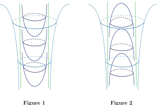
For this construction, we can choose any ofG_t,ψ_t, and Φ as in Construction 2.11. The above process including adding the positive side is the leafwise complex version of a turbulization. See also Figure 1 below.

2.2.3 General case

It is easy to find a closed transversal to a foliation of codimension one, namely, an embedded circle which is transverse to the foliation, unless the manifold

(11)

is open and the foliation is too simple. If we do not regard the leafwise complex structure, it is always possible to perform the turbulization in a tubular neighborhood of the closed transversal. However, even with leafwise complex structures, the situation is almost the same because of the following fact, which also belongs to folklores.

Theorem 2.13 Let (M²ⁿ⁺¹,F, J) be a smooth leafwise complex foliation of codimension one and K ⊂ M a closed transversal, namely there exists a smooth embedding f :S¹ → M which is transverse to the foliation F with its image f(S¹) =K.

Then, there exists a tubular neighborhood U ∼= K ×intD²ⁿ such that the restricted foliation (U,FU, J|FU) is isomorphic to the standard one (S¹× intD²ⁿ,F0 ={{t} ×intD²ⁿ}, J₀) and through this isomorphism, K is identified with S¹× {O}.

In particular, we can perform the standard turbulization 2.12 in U.

This theorem follows from the following lemma.

Lemma 2.14 The group Diﬀ^hol(Cⁿ, O) of germs of holomorphic diﬀeomor- phisms of (Cⁿ, O) which fix the origin is pathwise connected.

The lemma immediately follows from the two facts thatGL(n;C) is pathwise connected and that such a germ with identical linear part can be joined by a straight segment to the identity.

2.2.4 Dehn surgery in dim = 3 vs. higher dimensional turbulization

In order to close the section, this subsection provides with some remarks concerning the possibility of pasting the Reeb component in a diﬀerent way in a turbulization. In the rest of this section and in fact that of this thesis, let us assume the holonomy Ψ and thus accordingly φ and ψ as well to be tangent to the identity to the infinite order at the origin.

Remark 2.15 If we forget the leafwise complex structure and treat foliations only as smooth objects, basically there are two ways to perform the turbulization. The one has been already described above and is indicated in Figure 1. For the other one we can reverse the top and bottom of the Reeb component (Figure 2). This is because the cyclic (universal for n ≥2) covering of the boundary leaf is R²ⁿ \ {O} ∼= S²ⁿ \ {N, S} and two ends are exchangeable by a diﬀeomorphism. However, as a complex manifold, Cⁿ\{O}has one convex end and one concave. For the case of leaf dimension n is greater than 1, these two ends are not exchangeable. In particular, for n ≥ 2, the turbulization for leafwise complex foliations can not change the homotopy class of the tangent bundle.

(12)

Note that for these arguments we have to pay attentions only to complex structures of the boundary leaves, because we are dealing with flat structures.

Figure 1 Figure 2

The leaves indicated with green lines are the boundary leaves of Reeb components. If the reader imagine the axes of rotational symmetries of the figures, they correspond to {O} ×R+.

Remark 2.16 In the case of complex leaf dimension = 1, the ‘upside- down’ construction always works. Namely, in Construction 2.6, z ↔ z⁻¹ always induces an biholomorphic map on the boundary elliptic curve.

If the boundary elliptic curve admits a complex multiplication, namely finite but discrete symmetries of order 2, 3 or 4, removing the Reeb component and pasting it back with one of those symmetries is a special kind of Dehn surgeries.

More generally, in the turbulization, remove the Reeb component and first leave it. We prepare another Reeb component with a diﬀerent complex structure. If their boundaries match up through some diﬀeomophism, we can fill up the boundary with that Reeb component. In this way, a Dehn twist corresponding to any element of the mapping class group M1(∼= SL(2;Z)) of a 2-dimensional torus T² is realized for a closed transversal in a leafwise complex codimension one foliation of n = 1.

(13)

Chapter 3 Functional equations on flat functions

In this chapter some preliminaries for the determination of the automorphisms of a Reeb component concerning certain functional equations for flat functions which involve the holonomy diﬀeomorphisms.

Let φ ∈ Diﬀ^∞([0,∞)) be a diﬀeomorphism of the half line which is tangent to the identity to them-th (0≤n ≤ ∞) order at x= 0 and satisfies φ(x)−x > 0 for x > 0. Also we fix a complex number λ with |λ| > 1.

Let us consider the following (system of) functional equations on β, β₁ and β₂ ∈ C^∞([0,∞);C) concerning φ and λ. If λ is a real number, we can consider the same equations for β₂ ∈C^∞([0,∞);R).

Equation (I) : β(φ(x)) =λβ(x).

Equation (II) : β₁(φ(x)) =λβ₁(x) +β₂(x), β₂(φ(x)) =λβ₂(x).

First consider these equations on (0,∞). Then, Equation (I) has a lot of solutions. In fact, if we fix any solution β^∗ ∈ C^∞((0,∞);C) which never vanishes, i.e. β^∗(x) ̸= 0 for x > 0, then each solution corresponds to a smooth function on S¹ = (0,∞)/φ^Z by taking β → β/β^∗. This gives a bijective correspondence as vector spaces between the space Z = Zφ,λ of solutions to (I) on (0,∞) and C^∞(S¹;C).

Also take the space S = Sφ,λ of solutions to Equation (II) on (0,∞). If we assign β₂ to a solution (β₁, β₂)∈ S, we obtain the projectionP₂ :S → Z. Here the kernel of P₂ is nothing but Z. We also see that the projection P₂ is surjective because for any β2 ∈ Z

β₁(x) = 1

λlogλβ₂(x) logβ^∗(x)

gives a solution (β₁, β₂)∈ S, where for logβ^∗(x) any smooth branch can be taken. Therefore, as a vector space, S has a structure such that

0 → Z → S → Z → 0 is a short exact sequence.

(14)

3.1 Solutions for an infinitely tangent diﬀeo- morphism

In this section, we determine the spaces of solutions to the equations (I) and (II) for a diﬀeomorphism φ which is infinitely tangent to the identity at the origin. Key points of solving the equations are the infinite tangency ofφand the formula of Fa´a di Bruno.

Theorem 3.1 ([HM]) 1) Ifφ is infinitely tangent to the identity at x= 0, any solution β ∈ Z extends to [0,∞) so as to be a smooth function which is flat at x= 0, i.e. k-th jet satisfies j^kβ(0) = 0 for anyk = 0, 1, 2, · · ·.

2) The same applies to any solution (β₁, β₂)∈ S.

Remark 3.2 Let us consider the following system of functional equations on β₁ and β₂ ∈C^∞([0,∞);C) concerningφ, λ and a non-zero constantc.

Equation (IIc) : β₁(φ(x)) = λβ₁(x) +cβ₂(x), β₂(φ(x)) =λβ₂(x).

Let us take the spaceS(c) =Sφ,λ(c) of solutions to Equation (IIc) on (0,∞).

Then, by taking (β₁, β₂) 7→ (β₁, cβ₂), S(c) is in one-to-one correspondence with S. In particular, any solution (β₁, β₂) ∈ S(c) extend to [0,∞) so as to be smooth and flat at x= 0 by Theorem 3.1.

In the rest of this section we prove the above theorem. In order to clarify the strategy it might be suggested to the readers to check lim

x→+0β(x) = 0 and

xlim→+0β^′(x) = 0 i.e., for k = 0,1, which are almost trivial, and then the the second jet k = 2. Looking at the case k = 3 might make the roll of the following lemma clearer.

Lemma 3.3 The n-th derivative {β(φ(x))}⁽ⁿ⁾ is written in the following form for n∈N.

{β(φ(x))}⁽ⁿ⁾ = (φ^′(x))ⁿ·β⁽ⁿ⁾(φ(x)) +

n−1

∑

k=1

Φn,k·β^(k)(φ(x)).

Here, Φn,k is an integral polynomial in φ^′(x), φ^′′(x),· · ·, φ⁽ⁿ⁾(x), without constant term and no term is of monomial only in φ^′(x).

This lemma is easily seen by the induction, but in fact it is a corollary to the well-known formula of Fa´a di Bruno (e.g. see [Ri], [Ro], or textbooks on calculus). It is independent of our assumption on φ and is valid for any composite functions. On the other hand the flatness ofφat the origin implies (φ^′(x))ⁿ →1 and Φ_n,k →0 whenx→0 + 0.

Now let us prove 1) of Theorem 3.1. Letβ be a solution to (I) on (0,∞).

From the equation it is easy to see that β(x)→0 whenx→0 + 0.

(15)

Now fix any integer N. β^′(x) → 0 is also easy to see, but for higher derivatives, in a natural estimate the lower derivatives are involved. Thus the basic strategy is not to estimate the higher derivatives by induction on the order, but to estimate them all together up to the fixed order N.

From Equation (I) and the above lemma we have the following computa- tion.

∑N n=1

|β⁽ⁿ⁾(x)| = 1

|λ|

∑N n=1

{β(φ(x))}⁽ⁿ⁾

≤ 1

|λ|

∑N n=1

{

(φ^′(x))ⁿ· |β⁽ⁿ⁾(φ(x))|+

n−1

∑

k=1

|Φ_n,k| · |β^(k)(φ(x))| }

≤ 1

|λ|

∑N k=1

(

(φ^′(x))^k+

∑N n=k+1

|Φ_n,k| )

· |β^(k)(φ(x))|

As is remarked above, we know (φ^′(x))^k → 1 and ∑N

n=k+1|Φ_n,k| → 0 when x→0. Therefore there exists b_N >0 such that for x∈(0, b_N] we have

(φ^′(x))^k+

∑N n=k+1

|Φ_n,k| ≤√

|λ| for k = 1,2,· · · , N.

This implies for any x∈(0, b_N]

∑N n=1

|β⁽ⁿ⁾(x)| ≤ 1

√|λ|

∑N n=1

|β⁽ⁿ⁾(φ(x))|.

Put M = max{∑N

n=1|β⁽ⁿ⁾(x)|; x ∈ [b_N, φ(b_N)]} and define m_x ∈ N for x∈(0, b_N) so that φ^m^x ∈[b_N, φ(b_N)). Then, the above inequality implies

∑N n=1

|β⁽ⁿ⁾(x)| ≤M ·√

|λ|⁻^m^x

for x ∈ (0, b_N). Because ‘x → 0 + 0’ is equivalent to ‘m_x → ∞’, we obtain the convergence

β⁽ⁿ⁾(x)→0 (x→0 + 0) for n = 1,2,· · · , N.

This completes the proof of 1).

Let us outline the proof of 2). We extend the basic strategy of the proof of 1) in the following sense. When we estimate the derivatives of β₁, naturally those of β₂ are involved. Therefore we will estimate the derivatives of β₁ and β2 all together up to a fixed order N, even though the flatness of β2 is already proved in 1).

Reeb components of leafwise complex foliations and their symmetries