Bayesian parameter estimation using Gaussian states and measurements

states and measurements

Author Simon Morelli, Ayaka Usui, Elizabeth Agudelo, Nicolai Friis

journal or

publication title

Quantum Science and Technology

volume 6

number 2

page range 025018

year 2021‑03‑05

Publisher IOP Publishing Ltd.

Rights (C) 2021 The Author(s).

Author's flag publisher

URL http://id.nii.ac.jp/1394/00001855/

doi: info:doi/10.1088/2058-9565/abd83d

Creative Commons Attribution 4.0 International(https://creativecommons.org/licenses/by/4.0/)

PAPER • OPEN ACCESS

Bayesian parameter estimation using Gaussian states and measurements

To cite this article: Simon Morelli et al 2021 Quantum Sci. Technol. 6 025018

View the article online for updates and enhancements.

O P E N AC C E S S

R E C E I V E D

23 September 2020

R E V I S E D

30 November 2020

AC C E P T E D F O R P U B L I C AT I O N

4 January 2021

P U B L I S H E D

5 March 2021

Original content from this work may be used under the terms of the Creative Commons Attribution 4.0 licence.

Any further distribution of this work must maintain attribution to the author(s) and the title of the work, journal citation and DOI.

PAPER

Bayesian parameter estimation using Gaussian states and measurements

Simon Morelli^1,∗ , Ayaka Usui² , Elizabeth Agudelo¹ and Nicolai Friis¹

1 Institute for Quantum Optics and Quantum Information—IQOQI Vienna, Austrian Academy of Sciences, Boltzmanngasse 3, 1090 Vienna, Austria

2 Quantum Systems Unit, Okinawa Institute of Science and Technology Graduate University, Okinawa, Japan

∗ Author to whom any correspondence should be addressed.

E-mail:[email protected],[email protected],[email protected]and [email protected]

Keywords:quantum metrology, Bayesian estimation, Gaussian quantum optics

Abstract

Bayesian analysis is a framework for parameter estimation that applies even in uncertainty regimes where the commonly used local (frequentist) analysis based on the Cram´ er–Rao bound (CRB) is not well defined. In particular, it applies when no initial information about the parameter value is available, e.g., when few measurements are performed. Here, we consider three paradigmatic estimation schemes in continuous-variable (CV) quantum metrology (estimation of

displacements, phases, and squeezing strengths) and analyse them from the Bayesian perspective.

For each of these scenarios, we investigate the precision achievable with single-mode Gaussian states under homodyne and heterodyne detection. This allows us to identify Bayesian estimation strategies that combine good performance with the potential for straightforward experimental realization in terms of Gaussian states and measurements. Our results provide practical solutions for reaching uncertainties where local estimation techniques apply, thus bridging the gap to regimes where asymptotically optimal strategies can be employed.

1. Introduction

Quantum sensing devices hold the promise of outperforming their classical counterparts. However, since classical strategies can achieve arbitrary precision, provided that sufficiently many independent probes are used, the advantage of quantum sensing devices does not lie in the achievable precision. Instead, quantum strategies provide a faster increase in precision with n, the number of probes. In an idealised quantum sensing scenario, the estimation precision can in principle scale at the so-called Heisenberg limit (HL) of 1/n as n

→ ∞. In contrast, classical strategies can at most achieve a precision scaling of 1/√

n, the so-called standard quantum limit.

In the context of quantum optics, which we are interested in here, the possibility of preparing states with uncertain photon number means that the number of probes is uncertain. Therefore, the scaling usually refers to resources such as the mean photon number or mean energy of the probe systems. Nevertheless, general quantum strategies can result in a quadratic scaling advantage and thus outperform ‘classical’

strategies using the same resources. However, two important factors have to be considered.

First, preparing optimal or at least close to optimal probes and carrying out the corresponding joint measurements can be complicated and technologically demanding. Moreover, in the presence of

uncorrelated noise the scaling advantage with increasing n persists only up to a certain point, beyond which

only a (potentially high) constant advantage remains [1–3]. Even if one disregards any additional costs

that might incur from trying to combat noise [4,

5], overheads from complex preparation procedures and

the resulting low probe state fidelities may thus invalidate the expected benefits. Consequently, it is

important to identify estimation strategies that can outperform ‘classical’ approaches while being feasibly

implementable as well as robust against noise. For instance, for estimation problems in continuous-variable

(CV) systems, Gaussian states and measurements are generally considered to be comparably easily implementable. They allow achieving the HL for many scenarios within the local, also called ‘frequentist’, paradigm, including the local estimation of phases, displacements, squeezing and others [6–15].

Second, many of these insights are based on the Cram´ er–Rao bound (CRB). The CRB applies for estimation with unbiased estimators. It provides a lower bound for the precision via the inverse Fisher information (FI). Estimators that are unbiased locally (i.e., for specific parameter values) are readily available, but profiting from their unbiasedness requires precise prior information on the estimated parameter. The ‘local’ approach is therefore only well-justified when the number of independent probes is sufficiently large (hence ‘frequentist’), in such a case, the CRB provides the asymptotically achievable limit on scaling. However, when the available number of probes is limited (some authors [16–18] refer to

‘limited data’ in this context) then local estimation is not well defined. Resulting pathologies can lead to scaling seemingly better than the HL [19,

20] and even to an unbounded FI for finite average photon

numbers [21]. The available prior information also has to be carefully considered when calculating the CRB. For instance, for phase estimation with N00N-states, a growing (average) photon number n implicitly assumes that the prior interval is narrowing with 2π/n. If this is not accounted for, part of the scaling advantage comes from the increasing prior information, as pointed out in references [22,

23].

This motivates the study of Bayesian estimation approaches for quantum sensing, which we consider here. In Bayesian estimation, one’s initial knowledge of the parameter is described by a probability distribution (the prior) which is updated as more measurement data becomes available. The Bayesian approach is valid for an arbitrary number of probes and can in this sense be considered to be more rigorous than local estimation, at the cost of introducing a dependence on the prior. However, the influence of the prior vanishes for larger number of measurements, since the prior knowledge becomes less and less relevant with growing amount of measurement data. In practice, one may pursue a hybrid strategy, where initial Bayesian estimation is employed to sufficiently narrow down the possible range of the parameter before switching to a local estimation strategy with many repetitions.

Here, we consider Bayesian estimation scenarios for quantum optical fields. While much progress has been made for CV parameter estimation within the local paradigm, in particular, regarding the calculation of the quantum Fisher information (QFI) [6–9,

11–15] and the associated optimal strategies achieving the

CRB [24–29], CV parameter estimation in the Bayesian setting is much less explored. There, recent work has provided insight into Bayesian estimation with discrete [30] and CV systems using some specific probe states, including coherent states [16–18,

31],

N00N states [16,

32], and single-photon states [33].

Determining efficient and practically realizable strategies for Bayesian estimation in quantum optical systems can thus be considered an important link in the development of quantum sensing technologies, which this paper aims to establish.

Within the Bayesian paradigm, the additional freedom represented by the choice of the prior exacerbates the difficulty of determining optimal estimation strategies, making it all the more necessary to identify practically realizable strategies that can also be easily adapted. Here, in particular, we are interested in identifying strategies for Bayesian estimation considering Gaussian states and Gaussian measurements.

Gaussian states not only permit an elegant mathematical description in phase space, but are also especially easy to realise experimentally and are by now broadly used [34,

35]. Gaussian measurements, i.e.,

homodyne or heterodyne detection, have been shown to outperform number detection for few repetitions [17] and to be more robust against noise [27,

36,37] than photon number detection or ‘on/off’

detection—which discriminates only between the absence or presence of photons.

To broadly investigate the performance of Gaussian states and measurements in Bayesian metrology, we

consider three paradigmatic problems: the estimation of phase-space displacements, phase estimation, and

the estimation of single-mode squeezing. For each task, we provide practically realisable strategies based on

single-mode Gaussian states combined with homodyne or heterodyne detection that allow efficiently

narrowing the prior to the point where local estimation strategies may take over. To set the stage for this

investigation, we briefly review the method of Bayesian estimation and relevant concepts of Gaussian

quantum optics in section

2. In section3, we focus on the estimation of displacements for Gaussian priors,

and provide analytical results for the achievable precision using single-mode Gaussian states for both

homodyne and heterodyne detection. In sections

4

and

5, we proceed with similar investigations of Bayesian

estimation of phases and squeezing parameters, where we compare the performance of squeezing and

displacement of the probe system. Finally, we discuss our results and provide an outlook and conclusions in

section

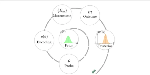
6.

Figure 1. Bayesian quantum parameter estimation. In Bayesian estimation scenarios, prior information encoded in a probability distributionp(θ) is updated based on available measurement data such as observing a particular measurement outcome m, resulting in a posterior conditional probability distributionp(θ|m). In quantum parameter estimation, the measurement procedure consists of preparing the system in a probe stateρon which the parameterθis encoded by a suitable transformation.

The measurement is represented by a positive-operator valued measure (POVM) with elementsE_mrepresenting the possible outcomes m.

2. Framework

In this section, we provide a brief overview of the relevant concepts in Bayesian estimation (section

2.1) and

Gaussian quantum optics (section

2.2), before we present our results in the following sections. For a more

extensive overview of classical Bayesian estimation theory we refer to [38–40], while more details on local and Bayesian estimation in the quantum setting can be found, e.g., in the appendix of [41].

2.1. Bayesian quantum parameter estimation

2.1.1. The Bayesian estimation scenario

The framework of Bayesian parameter estimation revolves around updating initially available information (or a previously held belief) based on new measurement data via Bayes’ theorem, as we will explain in the following. The initial knowledge of the estimated parameter θ is encoded in a probability distribution p(θ) called the prior distribution function or ‘prior’ for short. It captures all our beliefs (system properties, expertise) and information (prior experimental data) about the system under investigation. When a measurement is performed on the system, the probability p(m

|θ) to observe the measurement outcome

m in a system characterised by the parameter θ is called the likelihood, and can be calculated from the properties of the model used to describe the system and the measurement. Combined with the prior p(θ), the likelihood leads one to expect the outcome m with probability

p(m)

=

dθ p(m

|θ)

p(θ), (1)

where the integral is over the support of the prior and it is to be understood as a sum in case of a discrete parameter. The conditional probability that the estimated parameter equals θ, given that measurement outcome m was observed, can then be calculated via Bayes’ law, i.e.,

p(θ|m)

=

p(m

|θ)

p(θ)

p(m) . (2)

The function p(θ|m) is called the posterior distribution of the system parameter, after we have updated our belief with newly available data. The updating procedure, illustrated in figure

1, can be repeated arbitrary

many times, where the posterior of one step serves as the prior in the next step and the measurement procedure leading to p(m|θ) can in principle also be adapted from step to step.

After concluding the measurements, the posterior distribution represents a complete description of all

available information about the parameter. Nevertheless, it is often desirable (even if not strictly necessary)

to nominate an estimator θ

ˆ

and a suitable variance to express the result of the estimation procedure. While

the estimator assigns a specific value for θ to any prior or posterior, the variance quantifies the associated

uncertainty in the estimate. For parameters θ

∈R, the canonical choice for an estimator is the mean value

of the posterior distribution

θ(m)

ˆ =θ=

dθ p(θ|m) θ. (3)

In this case, a valid figure of merit for the confidence in this estimate is the variance of the posterior V

_post

(m)

=

dθ p(θ

|

m)

θ

−

θ(m)

ˆ 2

. (4)

A wide posterior with large variance suggests there is still high uncertainty in our belief about the parameter, whereas a narrow distribution with small variance indicates high confidence in our estimator.

Since the variance of the posterior generally depends on the measurement outcome, a good figure of merit for the expected confidence in the estimate provided by a particular measurement strategy is the average variance of the posterior,

V

¯post=

dm p(m) V

post

(m), (5)

which we will use here to quantify the precision of the estimation process. However, note that in some cases, the mean and mean square error variance above need to be replaced by more appropriate quantifiers. For instance, in the case that the parameter in question is a phase, where θ

=−π

and θ

=

π are identified, θ(m) and

ˆ

V

post

(m) can be replaced by suitable alternatives, as we will discuss in in section

4. In any given

setting, the task is then to determine estimation strategies that provide sufficiently high precision.

The precision of the estimation procedure generally depends on the shape of the prior, which can in principle be an arbitrarily complicated distribution. Uninformative priors generally influence the outcome less than narrow priors, so one should always be careful which amount of information should be encoded in the prior. However, the influence of the prior on the final estimate generally reduces with increasing

number of measurements, and can be argued to become irrelevant asymptotically, see, e.g., [38, chapter 13].

Consequently, encoding one’s knowledge only approximately using a family of probability distributions with only few degrees of freedom can help to facilitate a more straightforward evaluation of the performance of the chosen strategy, while preserving its qualitative features.

For instance, a class of probability distributions is said to be conjugate to a given likelihood function, if priors from within this class result in posterior distributions that belong to that class as well. Choosing the prior to be conjugate to the likelihood in this way makes the updating particularly easy, since this only requires the parameters to be updated to define the posterior distribution uniquely within the chosen class of probability functions, instead of requiring an entirely new calculation to determine the posterior.

Gaussian distributions are self-conjugate with respect to the mean, e.g. for Gaussian likelihood functions encoding the parameter to be estimated in their mean, the class of conjugate priors are Gaussian

distributions as well. The following proposition is a well known result in statistical theory [38–40,

42].

Proposition 1.

Let the likelihood be Gaussian distributed, p(m

|

θ)

=Nm

m(θ),

¯

σ

˜²

∝ Nθ

θ(m),

¯

σ

²

, where θ(m)

¯

is the mean of the distribution in θ, the parameter to be estimated. Then a Gaussian prior is the natural conjugate, i.e., if the prior is Gaussian distributed with p(θ)

=Nθ

(μ

0

, σ

₀²

), the posterior distribution p(θ|m) is also Gaussian with mean value μ

p=

σ

²

μ

0+

σ

²₀

θ(m)

¯

/(σ

²₀+

σ

²

) and variance σ

²_p=

(σ

²

σ

²₀

)/(σ

₀²+

σ

²

).

2.1.2. Bayesian estimation using quantum systems

The framework of Bayesian estimation can easily be applied to a quantum setting, as illustrated in figure

1.

In this case the parameter θ one is interested in estimating is encoded by a transformation that can generally be a completely positive and trace-preserving map. However, in many cases, including those we study here, the transformation is considered to be a unitary U

θ

that acts on an initially prepared probe state,

represented by a density operator ρ. The resulting encoded state is then given by ρ(θ)

=

U

θ

ρU

_θ^†

. The measurement of the encoded state can then be represented by a positive operator-valued measure (POVM) with elements E

m

0, whose integral (or sum in case of a discrete set of possible measurement outcomes m) evaluates to the identity on the Hilbert space of the probe, i.e., dm E

m=𝟙. In the quantum case the

likelihood is then given by p(m

|θ)=

Tr [E

m

ρ(θ)].

In local estimation scenarios with unbiased estimators θ, the CRB gives a lower bound for the variance

ˆ

of the estimator in terms of the inverse FI I

p(m|θ)

, that is, V( θ)

ˆ

I[p(m|θ)]

⁻¹

. Here, the FI depends only on the likelihood function and is given by

I p(m|θ)

=

dm p(m|θ)

∂

∂θ log p(m|θ)

2

. (6)

In the asymptotic limit of infinite sample size, the CRB is always tight, since it is saturated by the maximum likelihood estimator, which becomes unbiased in this limit, see e.g., [43]. Any local estimation problem can thus be reduced to determining an estimation strategy with a likelihood p(m|θ) corresponding to as large a FI as possible. In the quantum setting, this leaves us with the task of determining suitable probe states ρ and measurements

{

E

_m}m

. The optimisation of the FI over all POVMs can be carried out analytically, leading to the QFI

I

[ρ(θ)], and the corresponding quantum CRB [27,

44],

V( θ)

ˆ

1/

I

[ρ(θ)]. The QFI can be expressed in terms of the Uhlmann fidelity

F

(ρ

₁

, ρ

₂

)

=

Tr

√

ρ

₁

ρ

₂√

ρ

₁2

as

I

[ρ(θ)]

=

lim

dθ→0

8 1

−√

F

[ρ(θ), ρ(θ

+

dθ)]

dθ

²

. (7)

For the Bayesian estimation scenario, a similar bound exists. The Van Trees inequality bounds the average variance from below according to

V

¯_post

1

I p(θ)

+ ¯

I

p(m|θ) , (8)

where I p(θ)

=

dθ p(θ)

_∂

∂θ

log p(θ)

2

is the FI of the prior and

¯

I p(m

|θ)

=

dθ I p(m

|θ)

p(θ) is the average FI of the likelihood [45,

46]. This inequality is often referred to as the Bayesian CRB, see, e.g., [47].

In contrast to the CRB in the local scenario, this bound is not tight, which means there might not exist a strategy achieving the equality.

In a Bayesian quantum estimation problem, the Van Trees inequality can be modified to a Bayesian version of the quantum CRB by noting that the FI is bounded from above by the QFI,

I

[ρ(θ)] I p(m|θ)

. Moreover, if the parameter to be estimated is encoded by a unitary transformation U

θ

, the QFI is independent of θ. Consequently, the average FI can be bounded by the QFI to obtain the Bayesian quantum CRB

V

¯post

1 I

p(θ)

+I

[ρ(θ)] , (9)

which gives a lower bound for the average variance for all possible POVMs [41]. As before with equation (8), this bound is not tight.

While well-known methods for constructing optimal POVMs for fixed probe states exist for local estimation, optimization of the probe state and measurements for Bayesian estimation has to be carried out on a case-by-case basis and is typically challenging. At the same time, states and measurements that are optimal for a given prior may require complicated preparation procedures while generally no longer being optimal after even a single update. Consequently, it is of interest to devise measurement strategies for Bayesian estimation that are easily realizable and provide ‘good’ performance for different priors. Here, we provide and examine such strategies for a range of estimation problems in quantum optical scenarios.

2.2. Gaussian quantum optics

As we established before, we are interested in the analysis of scenarios where probe states are quantum states of the electromagnetic field. In particular, our goal is studying the performance of Gaussian states. To set the stage for this investigation, we will here briefly summarize the relevant concepts of Gaussian quantum optics. For a more extensive treatment of CV systems and Gaussian quantum optics we refer the reader to the references [48,

49] and for the particular context of quantum information processing cf references

[50–55]. Multimode optical fields can be represented as collections of bosonic modes. We consider a CV system that consists of N bosonic modes, i.e., N quantum harmonic oscillators. To each mode, labelled k, one associates a pair of annihilation and creation operators,

ˆ

a

k

and

ˆ

a

^†_k

, respectively. These mode operators satisfy the bosonic commutation relations [ˆ a

_k

,

ˆ

a

^†_l

]

=

δ

_kl

. The mode operators can be combined into the quadrature operators

ˆ

q

_k=

(ˆ a

_k+ ˆ

a

^†_k

)/

√

2 and

ˆ

p

_k=

i(ˆ a

^†_k−ˆ

a

_k

)/

√

2. These operators correspond to the generalized position and momentum observables for the mode k. They have continuous spectra, and eigenbases

{|q}q∈R

and

{|p}p∈R

, respectively. In the simplectic form [56], the quadrature operators are collected in one single vector

ˆx=

(ˆ q

1

,

ˆ

p

1

, . . . ,

ˆ

q

N

,

ˆ

p

N

)

^T

.

The state of such an N-mode system is described by a density operator ρ

∈ D

(

H^⊗N

), a positive

(semi-definite) and unit trace operator. Alternatively, the state of the system can be represented by its

Wigner function W(x) [57], i.e., a quasiprobability distribution in the 2N-dimensional phase space with real

coordinates q

_i

, p

_i∈R

, collected in a vector

x=

(q

₁

, p

₁

, . . . , q

_N

, p

_N

)

^T

.

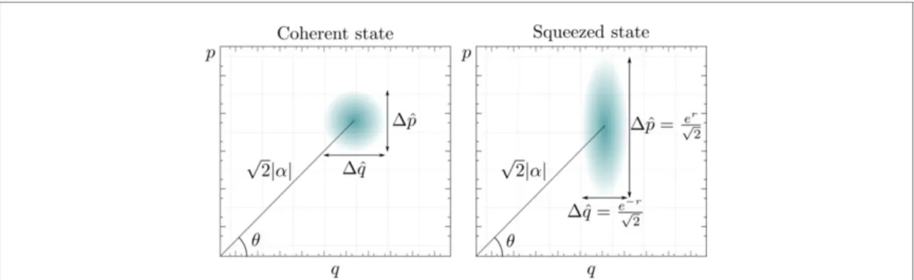
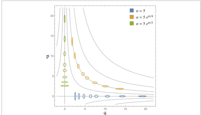
Figure 2. Contours of the Wigner functions for single-mode Gaussian states. The Wigner functions are given by Gaussian distributions of the form equation (10), and are characterised by a complex displacementα, a real squeezing strengthrand a squeezing angleϕ. The illustration compares a displaced vacuum state (r=0) on the left-hand side and a squeezed displaced state withr>0 andϕ=0 on the right-hand side. The width of the latter Wigner function is reduced in theˆq-quadrature and increased in theˆp-quadrature with respect to the coherent state.

2.2.1. Gaussian states

In the cases where the Wigner function of the state is a multivariate Gaussian distribution of the form W(x)

=

exp[−(x

−¯x)^TΓ⁻¹

(x

−¯x)]

π

^N√

det(Γ) , (10)

the states are called Gaussian. Gaussian states are fully characterized by its vector of first moments

¯

x=

Tr(ˆ

xρ) and its covariance matrix

σ

=

(σ

_ij

)

=¹₂Γ. The real and symmetric 2N×

2N covariance matrix collects the second moments σ

_ij={ˆx_i− ˆx_i

,

ˆx_j− ˆx_j}

/2. Examples for Gaussian states include the vacuum state, thermal states as used, e.g., to describe black-body radiation, or coherent states modelling the photon distribution in a laser. The full description via the vector of first moments and the covariance matrix allows one to completely and compactly capture an important class of familiar states in an infinite-dimensional Hilbert space via a finite number of degrees of freedom.

In this paper we investigate the performance of single-mode Gaussian states for Bayesian parameter estimation. More specifically, we consider coherent and displaced-squeezed states. Coherent states are the right-eigenstates of the annihilation operator

ˆ

a

_k

such that

ˆ

a

_k|

α

_k=

α

|

α

_k

and form a basis in the Hilbert space

Hk

. They result from applying the displacement operator of the coherent amplitude α

∈C,

D

ˆk

(α)

=

exp

αˆ a

^†_k−

α

^∗ˆ

a

k

, (11)

to the vacuum

|

0

_k

, such that

|

α

_k= ˆ

D

k

(α)

|

0

_k

. Coherent states are states with the same covariance matrix as the vacuum state. For a single-mode coherent state

|

α

_k

, the first moment is

¯x=√

2[(α),

I(α)]^T

and the second moment is the identity matrix divided by 2, meaning that the variance both in

ˆ

q

_k

and

ˆ

p

_k

equals 1/2, saturating the uncertainty relation in a balanced way.

Coherent states are not the only states saturating the uncertainty relation. Indeed, squeezed states are a larger class of states with this property, while allowing for unbalanced variances of the two canonical quadratures for each mode, cf figure

2. Squeezed states are obtained by the action of the squeezing operator,

ˆ

S

k

(ξ)

=

exp 1

2 (ξ

^∗ˆ

a

²_k−

ξˆ a

^†2_k

)

, (12)

on the vacuum

|

0

_k

. The states

ˆ

S

k

(ξ)| 0

_k

are characterized by a complex parameter ξ

=

re

^iϕ

, where r

∈R

is the so-called squeezing strength, and ϕ

∈

[0, 2π) is the squeezing angle.

Every pure single-mode Gaussian state has minimal uncertainty and can be generated by the combined action of squeezing and displacement operators on the vacuum state. Such states are therefore entirely specified by their displacement parameter α

∈C, their squeezing strength

r

∈R, and their squeezing angle

ϕ

∈

[0, 2π). If squeezing is restricted to a real parameter only, then also a phase rotation

ˆ

R

_k

(θ)

=

exp

−

iθˆ a

^†_kˆ

a

_k

, (13)

is needed to describe the most general pure single-mode Gaussian state. The vector of first moments of such a displaced squeezed state

|α,

re

^iϕ= ˆ

D(α)

ˆ

S(ξ)

|

0

= ˆ

D(α) R(ϕ/2)

ˆ ˆ

S(r)

|

0

is given by

¯x=√

2[ (α),

I(α)]^T

and its covariance matrix is σ

=

1

2

cosh 2r

−

cos ϕ sinh 2r sin ϕ sinh 2r sin ϕ sinh 2r cosh 2r

+

cos ϕ sinh 2r

. (14)

A unitary transformation is called Gaussian, if it maps Gaussian states into Gaussian states. This class of unitary operations is generated by Hamiltonians that are (at most) second order polynomials of the mode operators. Notice that every single-mode Gaussian unitary operation can be decomposed into displacement, rotation, and squeezing operations. In addition to having a relatively straightforward theoretical

description, Gaussian states and Gaussian transformations are also especially relevant in practice, since they are typically easy to produce and manipulate experimentally [34,

35].

2.2.2. Gaussian measurements

Any measurement can be described by a positive-operator valued measure (POVM). In CV quantum information, it is common to use continuous POVMs, that is, POVMs that are continuous sets of operators and a continuous range of measurement outcomes. A measurement is called Gaussian if it gives a Gaussian distribution of outcomes whenever it is applied to a Gaussian state. Gaussian measurements that are frequently considered in the context of CV quantum information are homodyne [58,

59] and heterodyne

detection [60]. Homodyne detection corresponds to the measurement of a mode quadrature, for example

ˆ

q.

In this case, the POVM consists of projectors onto the quadrature basis,

{|qq|}q∈R

. For heterodyne detection the POVM elements are projectors onto coherent states

{_π¹|

β

β

|}β∈C

. Moreover, we note that it has recently been shown that every bosonic Gaussian observable can be considered as a combination of (noiseless and noisy) homodyne and heterodyne detection [61].

3. Displacement estimation

We now consider Bayesian estimation of displacements using Gaussian states and Gaussian measurements.

That is, we assume a displacement operator D(α) as in equation (11) acts on our system, initially prepared

ˆ

in a Gaussian probe state. We then want to estimate the unknown displacement parameter α

=

α

R+

iα

I

, with α

R

, α

I ∈R

. To this end, we focus on estimation strategies based on heterodyne and homodyne detection. These measurements are covariant under the action of displacement in the sense that the probability distribution obtained by displacing the probe state gives the same probability distribution translated by the displacement parameter in the parameter space [62]. Without loss of generality, we can therefore assume that the initial probe state has not been displaced from the origin, i.e., that our probe state is a squeezed vacuum state

|ξ= ˆ

S(ξ)|0 with

ˆ

S(ξ) defined in equation (12). We further assume that our prior knowledge of the displacement is encoded in a Gaussian distribution of width σ

0

that is centered around α

₀

, i.e.,

p(α)

=

1 2πσ

₀²

exp

−|

α

−

α

₀|²

2σ

²₀

. (15)

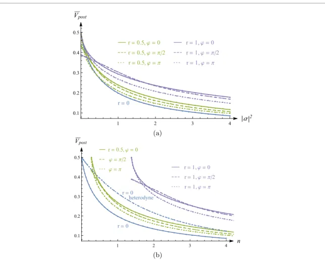
Our goal is then to examine the performance of the estimation strategies based on heterodyne and homodyne detection, including the respective asymptotic behaviour, both in the limit of high photon numbers and of repeated measurements, and compare the respective results.

3.1. Heterodyne measurement

Let us first consider heterodyne detection, where the measurement is described by the POVM

{¹_π|ββ|}β∈C

. The probability to obtain the measurement outcome β , given a displacement of α, is

p(β

|α)=

1 π Tr

|ββ|

D(α)

ˆ |ξξ|

D

ˆ^†

(α)

=

1 π

F

|β−

α ,

|ξ

. (16)

Here,

F

(ρ

1

, ρ

2

) is the Uhlmann fidelity of the states ρ

₁

and ρ

₂

(defined in section

2.1.2), which reduces to F

|ψ

,

|φ

=| ψ|φ |²

for pure states. For two Gaussian states, the fidelity can be written in terms of the respective first moments

¯x1

and

¯x2

, and second moments

Γ₁

and

Γ₂

(cf [7]) as

F

(ρ

₁

, ρ

₂

)

=

2 exp[

−

(¯

x₁−¯x₂

)

^T

(Γ

₁+Γ₂

)

⁻¹

(¯

x₁−¯x₂

)]

|Γ₁+Γ₂|+

(1

− |Γ₁|)(1− |Γ₂|)−

(1

− |Γ₁|)(1− |Γ₂|)

. (17)

For simplicity we now assume that our probe state is squeezed only along one fixed direction, i.e.,

ϕ

=

0. This simplifies the following calculation considerably. In particular, this allows us to write the

fidelity, the likelihood, and posterior distribution as products of the corresponding distributions for the real

and imaginary part of the displacements, respectively. In contrast, for the general case of probe states

squeezed along arbitrary directions, the resulting formulas are unwieldy and complicated, but qualitatively yield the same behaviour as for ϕ

=

0. We therefore refrain from presenting these calculations here.

In our case, we have ρ

1=|β−

αβ

−

α| and ρ

2=|ξξ|, for which the first moments are

¯

x_β−α=√

2

[β

−

α]

I[β−

α]

=√

2

β

_R−

α

_R

β

I−

α

I

and

¯xξ=

0

0

, while the second moments are represented by

Γ_β−α=𝟙2

and

Γξ=

e

^−2r

0 0 e

^2r

, respectively. Accordingly, p(β|α) from equation (16) becomes

p(β

|α)=

exp

−^{er(βR−αR)}_cosh^2+e−r_r^(βI−αI)2

π cosh r

=

p(β

R|αR

) p(β

I|αI

), (18) where the distributions p(β

_i|αi

) for i

=

R, I are given by

p(β

_i|αi

)

=

√

2 exp

−^2(β_1+eⁱ⁻∓2r^αi)2

√

π(1

+

e

^∓2r

) . (19)

Here and in the following equations, the upper and lower signs in

±

and

∓

correspond to the subscripts i

=

R and i

=

I, respectively, i.e., for i

=

R, the respective upper signs apply, while the lower signs apply for i

=

I. With this expression for the likelihood and with the prior from equation (15), one can use Bayes’ law [equation (2)] to calculate the posterior distribution, the estimators and the (average) variance. This allows one to evaluate the average variance for different estimation scenarios. We rely on such an approach in the next sections. However, in the special case where both prior and likelihood are Gaussian, these two

quantities are conjugate to each other. Following proposition

1, the posterior is therefore also Gaussian, and

we can write down the mean and variance of the posterior directly by inspecting the likelihood and the prior. That is, by noting that σ

²=

(1

+

e

^∓2r

)/4, μ

₀=

α

0,i

, and θ(m)

¯ =

β

i

, proposition

1

provides the mean and variance of the distributions p(α

_i|βi

). Again using subscripts i

=

R, I to denote real and imaginary parts, respectively, the means are

ˆ

α

_i

(β

_i

)

=

4β

i

σ

₀²+

α

0,i

(1

+

e

^∓2r

)

4σ

₀²+

1

+

e

^∓2r

, (20)

which we choose as estimators for the real and imaginary part of the parameter α, and the variances are Var[p(α

i|βi

)]

=

1

σ

₀²+

2(1

±

tanh r)

₋₁

. (21)

We then define the total variance of the posterior p(α|β ) for the complex parameter α as Var[p(α

|

β)]

=

dα p(α

|

β)

|

α

−

α(β)

ˆ |²

. (22)

Because the real and imaginary parts become independent, we can further write the total variance as the sum of the variances of the two independent estimation parameters, i.e.,

Var[p(α|β)]

=

Var[p(α

R|βR

)]

+

Var[p(α

I|βI

)]. (23) After inserting equation (21) twice, the latter expression is independent of β and therefore it already represents the average total variance V

¯post

we are interested in determining.

Moreover, it depends only on the variance σ

₀²

of the prior and the squeezing strength r of the probe state. For a fixed prior, the average posterior variance of both coordinates from equation (23) is minimized for r

=

0, that is, when there is no squeezing of the probe state. We thus have

V

¯_post

(r) V

¯_post

(r

=

0)

=

2σ

₀²

1

+

2σ

₀²

. (24)

However, squeezing can help to reduce the variance in one coordinate, but this reduction comes at the cost

of increasing the variance of the other coordinate with respect to the case where r

=

0. Irrespective of the

squeezing strength, we observe that the variances for both phase space coordinates decrease with respect to

the prior, but only slightly. When one is interested in reducing the variance in only one of the coordinates,

say α

R

, one may note that the variance decreases monotonically for increasing r. Nevertheless, even as r

→ ∞

the variance of the posterior is still bounded from below by (σ

₀⁻²+

4)

⁻¹

. This residual variance originates in the intrinsic uncertainty of the coherent-state basis associated with the POVM representing heterodyne detection. That is, no matter which measurement outcome is obtained, the precision with which the parameter is identified is limited by the width of the variance of the coherent state corresponding to this outcome.

Although coherent states already minimize the product of uncertainties, one can overcome this limitation by considering measurement bases that consist of states with a lower variance in the desired parameter (e.g., in α

_R

) than that of a coherent state, at the expense of a larger variance in the respective other quadrature. For instance, one may choose a basis of squeezed coherent states to reduce the

uncertainty of the measurement basis in one coordinate. In this regard, a homodyne measurement in the quadrature

ˆ

q, which we will consider next, can be thought of as a limiting case of a measurement in a basis of infinitely squeezed coherent states.

3.2. Homodyne measurement

For homodyne detection with respect to the quadrature

ˆ

q, the POVM is

{|

q

q

|}q∈R

. As before, we begin by considering a squeezed vacuum state

|

ξ

as probe state to estimate the unknown displacement α. The prior distribution of α is again assumed to be Gaussian with mean α

0

and variance σ

₀²

. The probability to obtain outcome q after a displacement α is given by

p(q

|α)=|

q

|

D(α)

ˆ |ξ|²=

exp

− ²

α_R−^√q

2 2 cosh 2r−cosϕsinh 2r

√

π(cosh 2r

−

cos ϕ sinh 2r) . (25) Note that, here, the likelihood does not depend on the imaginary part α

I

of the displacement. This is expected, since homodyne detection in one quadrature is completely ‘blind’ to the orthogonal quadrature.

Therefore, the mean and variance for the imaginary part of the displacement parameter remain unchanged with respect to the prior, and we can focus entirely on the real part.

Since, once again the likelihood is a Gaussian distribution in the measurement outcomes (here, in q), and thus proportional to a Gaussian distribution

Nα_R

(

α

_R

, σ

²

) in the estimated parameter with mean

αR=

q/

√

2 and variance σ

²=

(cosh 2r

−

cos ϕ sinh 2r)/4, we can infer from proposition

1

that the posterior is a Gaussian distribution with mean

ˆ

α

R=

2

√

2 σ

₀²

q

+

α

0,R

(cosh 2r

−

cos ϕ sinh 2r)

4σ

₀²+

cosh 2r

−

cos ϕ sinh 2r , (26)

and variance

Var[p(α

R|q)]=

σ

₀²

(cosh 2r

−

cos ϕ sinh 2r)

4σ

²₀+

cosh 2r

−

cos ϕ sinh 2r . (27)

The variance of the posterior distribution depends on the squeezing strength r and the squeezing angle ϕ. Both parameter hence provide room for optimization of the estimation procedure. However, while increasing r can be demanding experimentally and also comes at an increased energy cost for preparing the probe state, the relative angle ϕ between the directions of measurement and squeezing can be varied freely without any particular practical or energetic restriction. The variance is minimised for ϕ

=

2nπ and without loss of generality we choose ϕ

=

0. For this choice, the average variance of the posterior for the chosen quadrature

ˆ

q is

V

¯^ˆq_post=

Var[p(α

_R|

q)],

^ϕ=0=

, 1

σ

²₀ +

4 e

^2r −1

, (28)

whereas the average total variance (again, for ϕ

=

0) is V

¯_post= ¯

V

^ˆq_post+

σ

₀²

. Figure

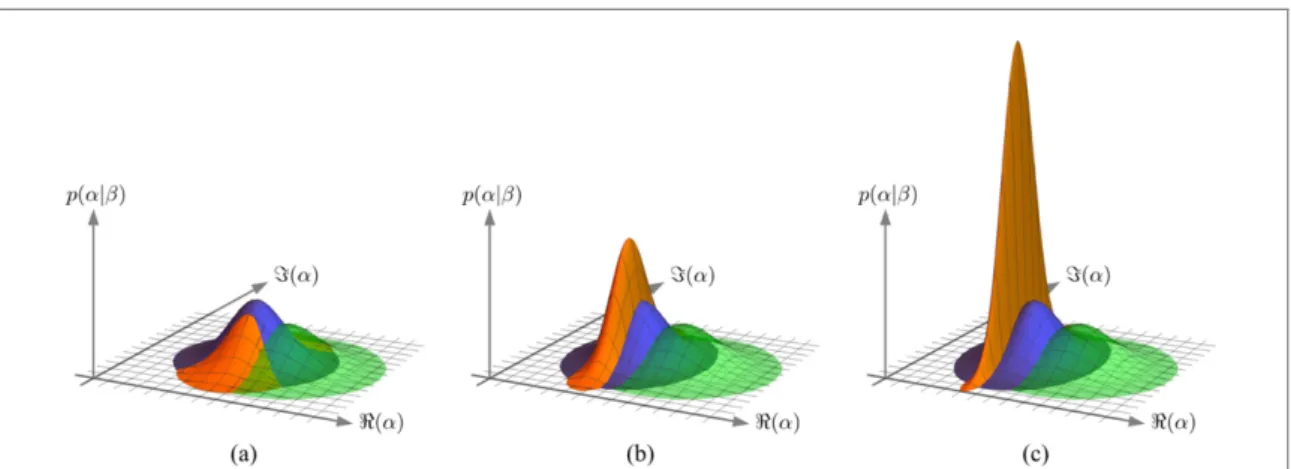
3

shows a sample of different posterior distributions obtained by measurements with probe states with different squeezing. We observe that, whereas the marginal probability in

ˆ

p remains unchanged as the initial squeezing increases, the marginal probability in

ˆ

q becomes narrower. We further note that for r

=

0 we recover the results obtained by Personick [63].

3.3. Comparison of measurement strategies

Let us now interpret and compare the results for Gaussian displacement estimation with heterodyne and

homodyne measurements. For homodyne detection, squeezing in the probe state results in an average

posterior variance in

ˆ

q, given by equation (28), that rapidly decreases to 0 as the squeezing strength r

increases. While the posterior variance in

ˆ

q can thus be arbitrarily close to zero in the homodyne detection

Figure 3. Displacement estimation using heterodyne and homodyne detection. The images show the same Gaussian prior (green) with initial standard deviationσ0=0.5, and posterior distributions obtained for heterodyne (blue) and homodyne detection (orange) for different squeezing of the probe state, ranging fromr=0 in (a),r=1 in (b), tor=2 in (c). The posterior distributions of the displacement parameterαgiven measurement outcomeqare Gaussian as well.

scenario, this comes at the cost of not reducing the variance in

ˆ

p at all. We thus have lim

_r→∞

V

¯^homodyne_post =

σ

₀²

. Comparing this with the result for heterodyne detection in equation (24), we see that V

¯^homodyne_post

V

¯^heterodyne_post

(r

=

0) for priors with variance σ

₀²

1/2, independently of the squeezing strength used with the homodyne detection. However, for more narrow priors, homodyne detection supplemented by squeezed probe states can outperform heterodyne detection in terms of the total variance only if the squeezing is strong enough, i.e., when r >

−¹₂

ln(1

−

2σ

₀²

).

However, when we focus on the estimation of only one of the quadratures, here quadrature

ˆ

q, then homodyne detection outperforms heterodyne detection for all prior widths and for all squeezing strengths, even if different squeezing strengths are compared for the two detection methods. That is, the limit of r

→ ∞

for heterodyne detection in equation (21) coincides with the homodyne detection case where r

=

0 in equation (28), and we thus find

V

¯^ˆq,homodyne_post

σ

²₀

1

+

4σ

₀²

V

¯^ˆq,heterodyne

post

. (29)

We can also compare these results to more general measurement strategies. For a Gaussian prior (in a single parameter), the FI of the prior (see section

2.1.2) evaluates to

I[p(α

_R

)]

=

1/σ

²₀

. At the same time, the QFI for a single-mode Gaussian state is bounded by

I

(ρ) 4 e

^2r

(cf equation (15) and subsequent text in reference [7]). With this, the Van Trees inequality in the form of equation (9) reads

V

¯^ˆq_post

1

σ

²₀ +

4 e

^2r ₋₁

. (30)

This shows that the combination of single-mode squeezing and homodyne detection is the optimal strategy for Bayesian estimation of one coordinate of displacement (or displacement radius with known phase) with a single-mode Gaussian probe state.

Finally, let us consider repeated measurements, which can easily be accommodated within the framework of conjugate priors. In particular, we know that the posterior is of the same form as the prior, i.e., both are normal distributions. Since the posterior distribution is used as the prior for the next measurement round, we obtain a recursive formula for the average variance, given by

σ

²_m+1=

σ

²_m

Var[p(q|α)]

σ

_m² +

Var[p(q

|

α)] , (31)

where σ

m

is the variance of round m. Since Var[p(q|α)]

=

e

^−2r

/4 depends only on the squeezing of the probe state, this term is constant for the same probe state. Solving the recursive equation gives

σ

_m² =

1

σ

₀² +

4m e

^2r ₋₁

. (32)

Moreover, we note that repeated measurements include the possibility of a sequential measurement strategy

that provides information about both components of the displacement. For instance, the squeezing in the

probe states and the direction of the homodyne measurement can be tailored towards estimating the real

part in one half of the estimation rounds, while the remaining rounds are used to estimate the imaginary part. We conclude this section by noting that already a quite simple setup, consisting of (limited) squeezing in the probe states combined with homodyne detection, can provide accurate information for Bayesian estimation of displacements.

4. Phase estimation

We now come to the paradigmatic case of phase estimation, which we want to examine within the framework of Bayesian estimation using Gaussian states and measurements. Historically, phase estimation has been closely associated with interferometry [64], but nowadays, phase estimation is usually considered in a broader context. In particular, Bayesian phase estimation has been studied for a variety of applications, see, e.g., [65–67]. While there are some studies identifying optimal estimation strategies using Gaussian states and measurements [15,

68,69], these operate within the local estimation paradigm and hence fall

outside of the Bayesian phase estimation framework we consider here. We therefore focus on a special case of Bayesian phase estimation, where there is no prior information on the phase and local estimation hence cannot be employed in a meaningful way. For such cases, we wish to identify simple strategies based on Gaussian states and measurements that can efficiently narrow the prior down to the point where local estimation can take over.

Specifically, we consider a phase estimation scenario where a phase rotation operator as in equation (13) is applied to a single-mode Gaussian probe state. We consider the phase θ

∈

[

−π,

π) to be entirely

unknown initially, such that the prior is a uniform distribution on the chosen interval, i.e., p(θ)

=

1/2π.

In the following sections, we then study the performance of heterodyne and homodyne detection in this estimation scenario, and we adapt the specific probe states to the respective measurements. In particular, we note that, although the optimal probe state (at fixed average energy) for local phase estimation is a

single-mode squeezed state, this is not necessarily the case for Bayesian estimation.

4.1. Heterodyne measurement

For Gaussian phase estimation with heterodyne measurements, we consider probe states that are squeezed with strength r

=|ξ|

before being displaced, i.e., probe states of the form D(α)

ˆ ˆ

S(re

^iϕ

)

|

0

, where r 0 and ϕ

∈

[0, 2π). Whereas the most general Gaussian single-mode probe states are determined by arbitrary complex values α and ξ, i.e., displacement and squeezing with arbitrary strength along arbitrary directions, the rotational symmetry of the phase estimation problem with heterodyne measurements allows one to fix one of these directions. Without loss of generality, we therefore choose α

=|

α

|

to be real and positive.

More specifically, we assume that the displacement is strictly non-zero, α > 0, since the vacuum state is rotationally invariant, and not even a squeezed vacuum state can be used to distinguish between rotations around θ and θ

+

π.

For the squeezing direction, it is then quite intuitive to see that squeezing along the quadrature

ˆ

p (ϕ

=

π, ξ

=−r

< 0) is optimal for single-mode phase estimation when α > 0 and when heterodyne measurements are used. That is, when the variance of the Gaussian state is initially reduced along the quadrature

ˆ

p, the Wigner function becomes concentrated along the

ˆ

q-quadrature, decreasing the variance in the phase of the initial state, and hence also decreasing the variance in the phase of the encoded state ρ(θ).

When applying the heterodyne measurement, the probability for obtaining an outcome β whose phase matches the unknown phase θ is thus increased. Conversely, probe states that are squeezed along the same direction as the initial displacement have an increased phase variance and are therefore less useful for phase estimation. In the remainder of this section, we therefore focus on probe states of the form D(α)

ˆ ˆ

S(

−

r)

|

0

.

However, since the calculations and results for arbitrary values of r are still quite unwieldy, we first consider the simple case where the probe state is not squeezed at all but just a coherent state

|α

(section

4.1.1). Then we present the results for squeezing along the optimal direction,

ξ

=−

r < 0, with respect to the displacement α > 0 (section

4.1.2).

4.1.1. Coherent states & heterodyne detection

Here, the probe state is

|α

with α > 0. The action of the phase rotation operator R(θ) [equation (13)]

ˆ

results in the encoded state R(θ)

ˆ |α=|e^−iθ

α. The likelihood to obtain outcome β

∈C, given that the

phase has the value θ, is given by

p(β

|θ)=

1

π

| β|e^−iθ

α |

² =

1

π e

^{−|eiθβ−α|2}

. (33)

Writing β

=|β|e^−iφβ

and

|e^iθ

β

−

α|

²=

α

²+|β|²−

2α|β| cos(θ

−

φ

_β

), we can express the (unconditional)

probability to obtain outcome β as p(β)

=

π

−π

dθ p(θ) p(β

|θ) =

e

^{−(α2+|β|2)}

π I

0

(2α|β|), (34)

where I

0

(x) is the modified Bessel function of the first kind. Using Bayes’ law, the posterior is given by p(θ|β)

=

p(θ) p(β

|

θ)

p(β)

=

e

2α|β|cos(θ−φ_β)

2π I

0

(2α|β|) . (35)

Since we are considering a parameter with a range whose endpoints

±

π are identified, it is useful to consider estimators and variances that are invariant under shifts by 2π. For the estimator we therefore choose θ(β

ˆ

)

=

arg

e

^iθp(θ|β)

. As we discuss in more detail in appendix

A.1, the estimator evaluates to

θ(β

ˆ

)

=

arg

⎡

⎣ π

−π

dθ p(θ|β)e

^iθ

⎤

⎦ =

φ

β

, (36)

and hence corresponds to the phase φ

β

of the measurement outcome β.

To evaluate the performance of this estimation strategy, we calculate the average variance of the posterior as done in the above sections. However, instead of an expression such as in equation (4), we now use a covariant variance that is invariant under shifts by 2π, by taking the average of sin

²

θ

−

θ(β)

ˆ

rather than of

θ

−

θ(β)

ˆ 2

.

³

Specifically, we calculate

V

_post

(β )

= π

−π

dθ p(θ

|β

) sin

²

θ

−

θ(β

ˆ

)

= ⁰

F

₁

(2; α

²|

β

|²

)

2 I

0

(2α|β|)

Γ(2)

, (37)

where

₀

F

₁

(a; z) is the confluent hypergeometric function and

Γ(z) is the Euler gamma function. Despite the

complicated form of the posterior and the variance, the average variance then simply becomes

V

¯post=

d

²

β p(β ) V

post

(β )

=

1

−

e

^−|α|2

2

|α|²

, (38)

as we discuss in more detail in appendix

A.1. In terms of the average photon number

n

=|α|²

, which is proportional to the average energy of the probe state, the average variance of the posterior hence scales as 1/n as n

→ ∞

, as can be expected for ‘classical’ probe states such as the coherent states considered here.

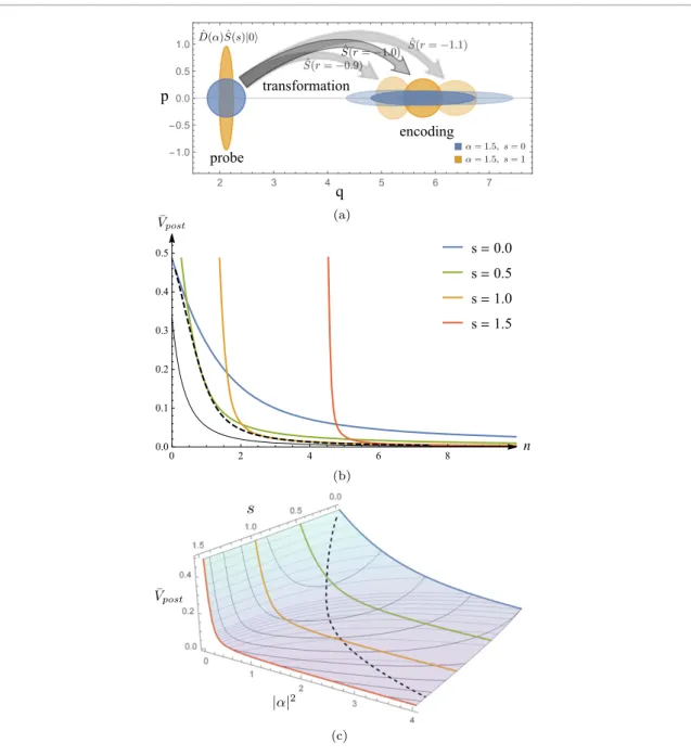
4.1.2. Displaced squeezed states & heterodyne detection

Let us now consider probe states that are squeezed with strength r before being displaced, i.e., probe states of the form D(α)

ˆ ˆ

S(

−

r)

|

0

, where we assume α, r

∈R

with α > 0 and r > 0 as mentioned. For the heterodyne measurement, the likelihood to obtain outcome β given the phase θ is given by

p(β

|θ)=

1

π

| β|

R(θ)

ˆ

D(α)

ˆ ˆ

S(−r)

|0 |²=

1 π

F

|e^iθ

β ,

|α,−r

. (39)

For the fidelity of the two Gaussian states, we can again refer to equation (17), where ρ

1=|e^iθ

βe

^iθ

β| and ρ

₂=|

α,

−

r

α,

−

r

|

, for which the first moments are

¯

x1= ¯x_eiθβ=√

2

(e^iθ

β)

I(e^iθ

β)

and

¯x2= ¯x_α,−r=√

2

(α) I(α)

.

The second moments of these states are represented by

Γ₁=Γ_eiθβ=𝟙2

and

Γ₂=Γ_α,−r=

e

^2r

0 0 e

^−2r

,

3We note here that the chosen variance is invariant also under shift of the estimator by integer multiples ofπ, not just shift by even multiples ofπ. In principle, one could also use quantifiers for the width of the distribution that depend only on|e^iθp(θ|β)|, such as the Holevo phase variance [70], which are completely independent of the value of the estimator. The choice we make here is motivated by the better comparison with the homodyne detection scenario in section4.2, where the phase can only be resolved within an interval of lengthπ.