A s t r uc t ur al anal ys i s of J apanes e ec onom
i c
devel opm
ent
著者
Ts uj i m
ur a Kaz us uke, Ts uj i m
ur a M
as ako
権利
Copyr i ght s 日本貿易振興機構(ジェトロ)アジア
経済研究所 / I ns t i t ut e of D
evel opi ng
Ec onom
i es , J apan Ext er nal Tr ade O
r gani z at i on
( I D
E- J ETRO
) ht t p: / / w
w
w
. i de. go. j p
j our nal or
publ i c at i on t i t l e
I D
E D
i s c us s i on Paper
vol um
e
695
year
2018- 02
INSTITUTE OF DEVELOPING ECONOMIES
IDE Discussion Papers are preliminary materials circulated
to stimulate discussions and critical comments
Keywords: Priority production system; Specialty financial institutions; Saving-
investment balance; Robotization.
JEL classification: C82; E16; O11
* Rissho University, Tokyo, Japan, e-mail: [email protected]
IDE DISCUSSION PAPER No. 695
A Structural Analysis of Japanese
Economic Development
Kazusuke TSUJIMURA and
Masako TSUJIMURA*
February 2018
Abstract
The Institute of Developing Economies (IDE) is a semigovernmental,
nonpartisan, nonprofit research institute, founded in 1958. The Institute
merged with the Japan External Trade Organization (JETRO) on July 1, 1998.
The Institute conducts basic and comprehensive studies on economic and
related affairs in all developing countries and regions, including Asia, the
Middle East, Africa, Latin America, Oceania, and Eastern Europe.
The views expressed in this publication are those of the author(s). Publication does
not imply endorsement by the Institute of Developing Economies of any of the views
expressed within.
I
NSTITUTE OF
D
EVELOPING
E
CONOMIES
(IDE), JETRO
3-2-2, W
AKABA
,
M
IHAMA
-
KU
,
C
HIBA
-
SHI
C
HIBA
261-8545, JAPAN
©2018 by Institute of Developing Economies, JETRO
No part of this publication may be reproduced without the prior permission of the
A Structural Analysis of Japanese Economic Development
Kazusuke Tsujimura
*
Masako Tsujimura
†
February 2018
Abstract
Japan successfully escaped from poverty after the world war and attained prosperity in a
matter of two decades. There were two keys for the success. One was the priority
production system
–
the idea to develop the industries at the bottom of the triangulated
input-output table first, and to climb the triangle step by step. The second key for the
success was the country’s unique financial system; they deliberately grew both long
-term
financial institutions for large enterprises and local credit associations for small
businesses. When Japanese exporting manufacturers fought the appreciation of yen at the
end of the 20th century, their answer was the mass introduction of industrial robots. The
exporters won the fight but the country did not. What went wrong; what lesson do we
learn from it?
Keywords: Priority production system; Specialty financial institutions;
Saving-investment balance; Robotization.
JEL: C82; E16; O11
*
Keio University, Tokyo, Japan
1
1. Introduction
After the financial crisis of 2008-2009, the interest rates of the mature economies
declined significantly while those of the developing economies remained high.
Therefore, large-scale fundraisers of the emerging markets turned to the major
economies for loans. The problem is that the gap in fundraising cost between the big
and small businesses is damaging the latter. Another problem is that the
dollar-denominated interest rate is creeping up as the U.S. economy recovers. Soon or later,
the developing countries will find it costly to depend on funds from abroad. It must be
a good idea for a developing economy to plan ahead and draw a design for self-sufficient
development both in terms of production and financing.
When the World War II ended, Japan was suffering from poverty; all the cities
were reduced to ruin. Soon after the war, Japan embarked on a project christened
‘priority production system’, which resembles to the Leontief’s economic development
2
3
economy from further deterioration by promptly injecting the incoming funds. The
unique system of long-term finance completely disappeared after the turn of the century.
Another set of specialty financial institutions that solely serve households and
small businesses were also set up in the postwar Japan in addition to more than a hundred
regional and mutual banks
1
. The staff of mutual banks used to regularly visit the
depositors to collect monthly installments; all the mutual banks switched to regional
banks by the end of 1980s. Japan consists of 47 administrative regions called
prefectures; each of them had at least one regional bank and one mutual bank. Each
prefecture consists of dozens of cities, towns and villages. Each city and town typically
had one credit union and one credit cooperative. The members of the credit unions and
credit cooperatives contribute deposits and the institutions provide loans and other
financial services to the members, most of them are small business owners. Agricultural
and fishery cooperatives, which has dense network of branches in rural area, also accept
deposits and make loans. Most of these institutions are still active in business in
21st-century Japan. One of the features of these smaller financial institutions are that each of
the category group has its own financial networks and headquarter that serves as a hub.
For example, the bank for credit unions known as Shinkin Central Bank, collects
redundant deposits from the credit unions and loans to the unions in need. The Bank of
Commerce and Industry, known as Shoko Chukin Bank in Japan, is an independent
semi-public bank serving small businesses.
2. Changes in the Industrial Structure
2.1 Overview
4
The growth in Japanese GDP during the latter half of the twentieth century is
depicted in Figure 1. While the black line represents nominal GDP (i.e. GDP at current
prices), the grey line indicates real GDP (GDP at 1990 prices). Both nominal and real
GDP grew steadily between 1955 and 1998. Real GDP tumbled in 1974 in the wake of
the oil crisis. In this year, not only the crude oil embargo by the Organization of Arab
Petroleum Exporting Countries but also the worldwide crop shortage caused by El Niño
immediately followed by La Niña
2
hit the Japanese economy; Japan suffered from
stagflation, a combination of stagnation and imported inflation. Real GDP dipped again
in 1998, however, at this time nominal GDP also slipped. In this year, the government
started to deregulate the Japanese financial markets, leading to restructuring of the way
those markets operate; long and short term financial markets were merged, and the
concept of universal banking was introduced. Yamaichi Securities, one of the top
security dealers, and Hokkaido Takushoku Bank, one of the top banks, consecutively
closed their doors for business. It took almost twenty years for the nominal GDP to reach
the previous maximum recorded in 1997. Figure 2 illustrates the composition of nominal
GDP. In 1955, the share of the primary industries, agriculture, forestry, fishing and
mining, was almost 22%; manufacturing accounted for 28%, and the other industries
held a share of a little less than 50%. The portion of the primary industries declined
steadily since then, and fell below 10% in the late 1960s, and below 5% around 1980
before reaching less than 2% in 1997. The share of manufacturing peaked in 1961 at
2
A backflow of the Trade Wind in the tropical Pacific Ocean that persists for several months or
5
36%, and remained at the level before the oil crisis battered the industry in 1973-74. The
share of manufacturing in nominal GDP rapidly dropped in 1975 and again in the
beginning of 1990s. Other industries including commerce and services accounted for a
little less than 50% in 1955, and increased its share in nominal GDP thereafter. The share
slightly shrank during recessions when nominal GDP growth rate dropped, however,
rapidly rose immediately after the oil crisis.
The decline in the share of agriculture in nominal GDP reflects the reduction in
employment, which is depicted in Figure 3.
While agriculture’s share in nominal GDP
was less than 22%, that in total employment was more than 36% in 1955 so that the
productivity was relatively low creating poverty in rural areas. The redundant labor
force was absorbed mainly by the manufacturers during the 1950s and 1960s, but by
other industries, which include construction, retail and wholesale, and other services,
after the 1970s. The share of manufacturing in employment quickly rose during 1960s,
however, suddenly dropped in 1975 in the aftermath of the oil crisis. Although the share
of manufacturing remained unchanged until 1992, it continuously declined thereafter
partially because of the recession that took place after the real estate bubble of late 1980s
collapsed. Most probably, another reason for the decline is the mass introduction of
industrial robots. The number of robots in operation in Japan
3
was 93 thousand in 1985,
but increased to 274 thousand in 1990 and then 387 thousand in 1995; more than 60%
of the world’s inventory of industrial robots were working in Japan
4
. These robots
quickly overtook the manufacturing jobs, assembling, painting, welding and packing
etc., from the laborers.
3
Data source: Japan Robot Association.
6
2.2 Input-Output Table
The first Japanese input-output table for 1951 was published by the Ministry of
International Trade and Industry, which covered 182 industries. The Japanese
government ministries have jointly produced input-output accounts since 1950s; the first
table was published for 1955 and every five years since then. We have prepared 1965
and 1995 tables for comparison based on the publication. Since the Japanese
input-output table is based on cost accounting, a row represents a product while a column
stands for a production activity. The original matrices we had used were 156
156 for
1965 and 186
186 for 1995 respectively
5
, however, we made 129
129 matrices for
each year to make direct comparison possible. Actually, 1995 table is extended to a 131
131 matrix to accommodate two newborn
industries: ‘computer and electronic
devices manufacturing’ and ‘industrial robot manufacturing’.
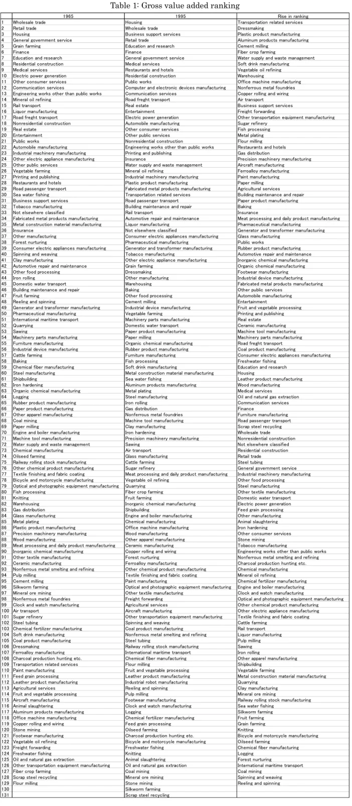
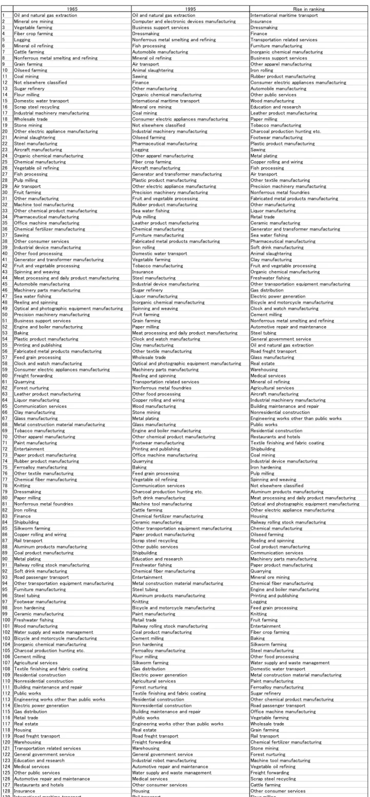
Table 1 lists the industries in order of gross value added. Wholesale and retail
trade are ranked high in both 1965 and 1995 and so are the service industries. However,
the last column reveals that the manufacturing industries performed far better in 1995.
It should be noted that ‘computer and electronic devices manufacturing’ is already
ranked at 12th place in 1995 even ab
ove the ‘automobile manufacturing’.
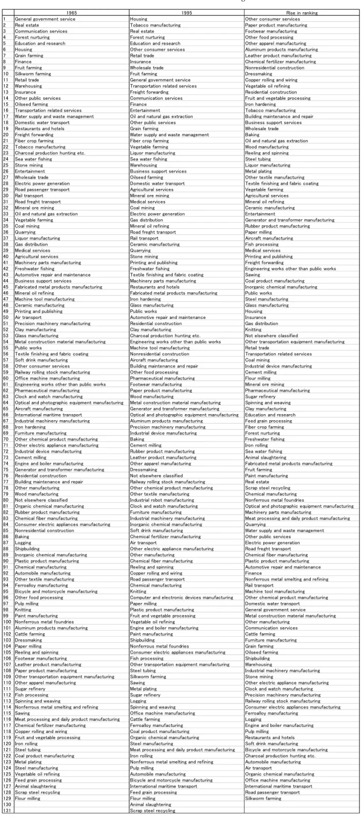
In terms of
the value added ratio, which is the ratio of gross value added to the total output of the
product, primary industries along with the real estate business that includes imputed rent
are ranked high in Table 2. Again, many of
the manufacturing industries’ ranking had
risen during the thirty years between 1965 and 1995. It is interesting to know, however,
the value added ratio of the automotive manufacturers, the main Japanese exporter, is
relatively low comparing to other industries. The ranking was 92nd in 1965 and was
7
even lower in 1995; it ranked 125th among 131 industries. The value added ratio
rankings for the newborn industries
were not much higher; ‘computer and electronic
devices m
anufacturing’ ranked 96th while ‘industrial robot manufacturing’
ended at
80th. Since gross value added includes indirect taxes etc., we compare the industries in
the ranking of compensation-of-employees ratio, which is the ratio of compensation of
employees to the total output of the product, in Table 3. Transportation and
communication services were ranked high both in 1965 and 1995 alongside ‘general
government service’ and ‘
e
ducation and research’.
The industries that raised their ranks
between the two years
included ‘food processing’ and
textile and apparel manufacturing,
which were considered to be declining industries by the end of the century; most
probably, they lost their competitiveness because of the high labor cost.
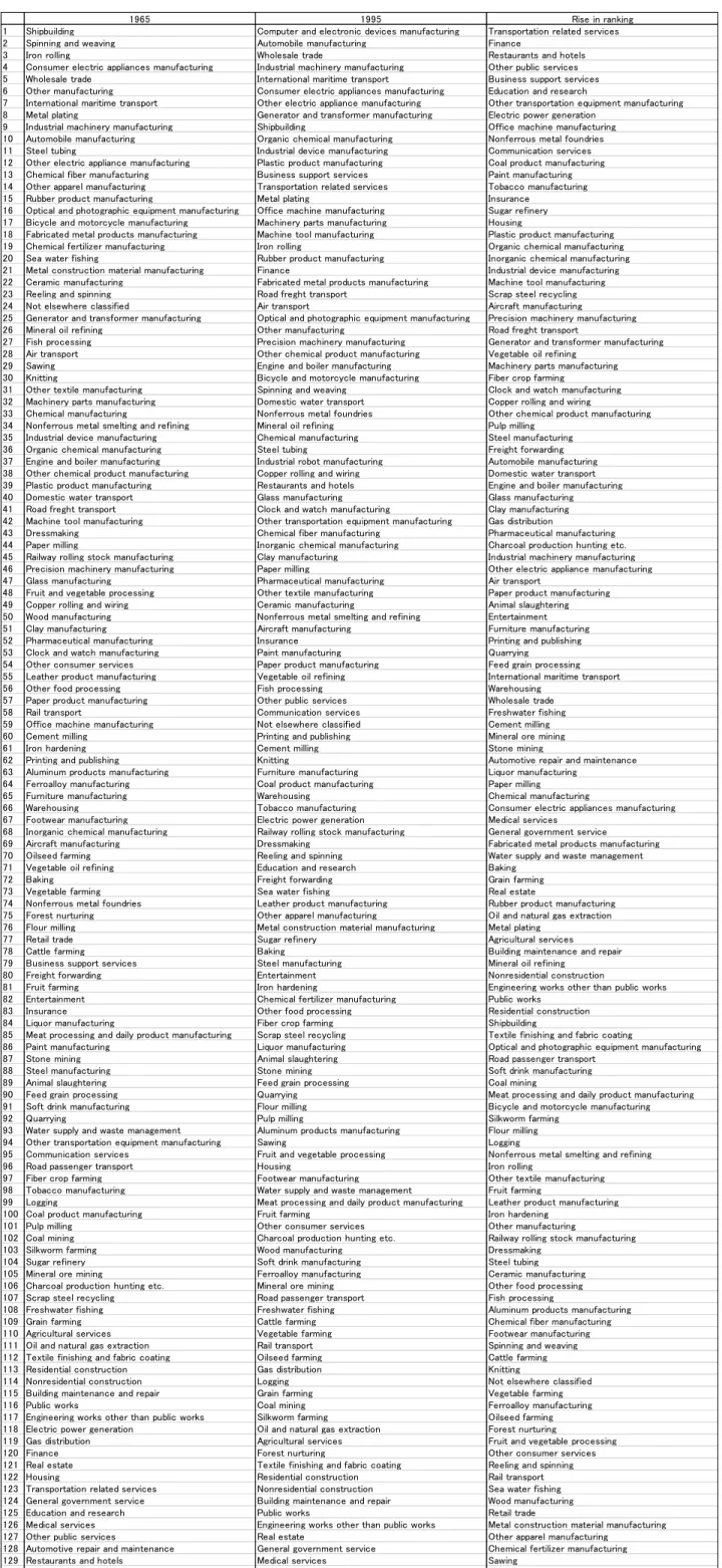
Table 4 lists the industries in order of the amount of exports. ‘Shipbuilding’ and
‘
spinning and
weaving’ lead the list
in 1965 followed by
‘iron and steel production’ and
‘consumer electric appliances manufacturing’.
However, by
1995, ‘computer and
electronic devices manufacturing’ and ‘automobile manufacturing’ had replaced the two.
Most of the industries that climbed the list between 1965 and 1995 were business
services, such as ‘transportation related services’ and ‘finance’.
Although, in 1965,
‘shipbuilding’ was also ranked first in the list of export ratio,
Table 5, the proportion of
exports out of total output of the product, ‘international maritime transport’ had replaced
it by 1995.
‘Industrial robot manufacturing’, the new
comer, was already fifth in the
ranking in 1995. Again, many of business services climbed the list between 1965 and
1995. Table 6 lists the industries in order of the amount of imports. In both 1965 and
1995, ‘oil and natural gas extraction’ ranked first a
s expected for a country that lack
8
‘computer and electronic devices manufacturing’ was ranked second in 1995.
Since
‘computer and electronic devices manufacturing’ was the large
st exporter in that year, it
seems that international fragmentation of production was already in progress in the
industry. It is also noteworthy that ‘dressmaking’ along with
business and financial
services climbed the ranking between 1965 and 1995. While
‘dressmaking’ was 79th in
the import ranking in 1965, it became 4th in 1995 implying that Japan was quickly losing
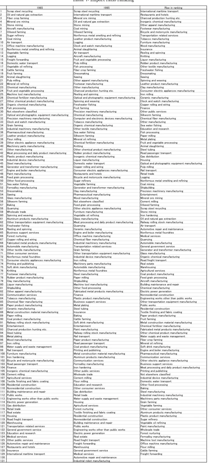
ground in handworks. As for the import ratio displayed in Table 7, which is the
proportion of imports to the total domestic demand, ‘scrap steel recycling’ topped the
list both in 1965 and in 1995. ‘Oil and natural gas extraction’ lowered its rank from the
2nd to the 4th as a result of intensive energy-saving investments after the oil crises of
the 1970s.
2.3 Triangulation
As Leontief (1963) asserts, one of the best tools to depict the industrial structure
(or hierarchy) of an economy is the triangulated input-output table. Triangulation is a
technique to simultaneously rearrange the rows and columns of the intermediate
transaction matrix of an input-output table so that the largest number of non-zero cells
fall below the diagonal running from the upper left corner to the lower right corner of
the matrix. “In the hierarchical order of an economy with a strictly triangular mat
rix, the
9
indirect demand for the output of the sector in question.” (
Ibid
. p. 153) “The e
xtent to
which the actual economy departs from one-way interdependence is indicated by the
proportion of transactions which fall above the diagonal in the optimal arrangement.”
(Chenery and Watanabe, 1958, p.494) Many algorithms of triangulation have been
proposed since late 1950s. For example, the procedure of Chenery and Watanabe is a
trial and error method of ranking the sectors corresponding to the ratio of inter-industrial
input to total input or inter-industrial output to total output. In this paper, however, we
are to use much simpler method of triangulation; just count the number of non-zero cells,
and rearrange the order of rows and columns accordingly.
Let
z
C
be a vector whose elements are the number of non-zero cells in each
column; and
z
R
be a vector whose elements are the number of non-zero cells in each
row. We further define
R
C
m
z
i z
z
(1)
where
m
is the number of rows and columns of the matrix, and
i
is a vector in which
all of the elements are 1. There are three alternative methods of triangulation. (i)
Triangulation according to the number of non-zero cells in each column; i.e. sort the
rows and columns in the descending order of
z
C k
, which is the
k
th element of vector
C
z
. (ii) Triangulation according to the number of non-zero cells in each row; i.e. sort
the rows and columns in the ascending order of
z
Ri
, which is the
i
th element of vector
R
z
. (iii) Triangulation according to the number of non-zero cells in the lower-left
10
which is the
i
th element of vector
z
. In method (i), the number of non-zero cells
above the diagonal was 31.3% for 1965 and 39.3% for 1995. In method (ii), the numbers
were 19.2% for 1965 and 22.6% for 1995; in method (iii), the numbers were 18.5% for
1965 and 22.1% for 1995. As far as the proportion of non-zero cells to the total number
of cells above diagonal is concerned, method (iii) is the best method of triangulation as
easily predictable. However, each of these methods has slightly different economic
implication. As we have mentioned already, Leontief (1963) found input-output
hierarchy in triangulation; the rows below are suppliers, and the rows above are
consumers of a particular product. Most probably, method (i) best serves the purpose
because it is the triangulation based on the input structure. Method (ii) is the
triangulation based on the output structure; the industries at the bottom of the triangle
supply their products to more industries than the industries above. The priority
production system, to which we have mentioned at the beginning of this paper, is based
on the idea. If we have a choice, we must develop the industries from the bottom up to
the top of the triangle obtained by method (ii). Meanwhile, as Leontief (1963) alluded,
the economic hierarchy is more conspicuous in a primitive economy than in a complex
economy, in which production processes are fragmented. Method (iii) must be the best
tool to know the degree of fragmentation; as Chenery and Watanabe (1958) suggested,
the proportion of non-zero cells above the diagonal might be a good indicator. We can
confirm from the above observations that the fragmentation certainly progressed in the
Japanese economy during the thirty years between 1965 and 1995.
11
very bottom of the triangle
were ‘finance’, ‘insurance’, ‘retail trade’, ‘wholesale trade’
and ‘transportation related services’ in that order. In 1995, ‘electric power generation’
and ‘mineral oil refining’ were among the five. In 1965, the industries at the top of the
triangle were
‘nonresidential construction’, ‘residential construction’, ‘engineering
works other than public works’, ‘public works’
and ‘automobile manufacturing’ in that
order. ‘General government service’ and ‘restaurants and hotels’ replaced ‘engineering
works othe
r than public works’ and ‘automobile manufacturing’ in 1995.
The industries
lowered
in triangulation ranking between 1965 and 1995 were ‘
education and research
’,
‘entertainment’, ‘freight forwarding’, ‘clock and watch manufacturing’ and ‘furniture
manufact
uring’. The industries rose in triangulation ranking were ‘transportation related
services’, ‘automotive repair and maintenance’, ‘general government service’ and
‘bicycle and motorcycle manufacturing’.
The industries at the bottom of the triangle are
casually know as upstream industries while those at the top are often called downstream
industries. Actually, there are no drastic changes in the triangulation order between 1965
and 1995. Most of upstream industries are either commerce, services for businesses or
public utilities, such as electric power generation and water supply. Row material
manufactures are at middle stream. Downstream industries include assembly
manufacturing, construction and services for consumers. Since, downstream industries
are relatively labor intensive, the urbanization of Japan was only possible, when the
bottom up industrialization under the priority production system reached this stage in
early 1960s.
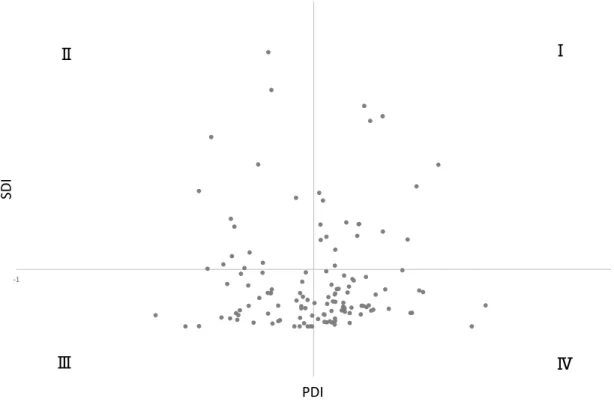
2.4 Dispersion Indices
12
also often used as industrial structure indicator. The power of dispersion index (PDI)
represents the column sum of Leontief inverse matrix while the sensitivity of dispersion
index (SDI) symbolizes the row sum. Since the Japanese input-output tables are of
Chenery-Moses type, the final demand includes imports with negative signs. Therefore,
we will use
A
M
I
I
M A
1instead of
A
I
A
1as Leontief inverse,
where I is a unit matrix, A is the input coefficient matrix, and M is a diagonal
matrix whose elements are import coefficients. While
A
represents technological
relationship between industries,
A
Mdepicts the industrial structure of an economy
taking the import coefficient, the ratio of import to the total domestic demand for the
product, into consideration. According to Rasmussen
’s
(1957, p. 134) definition, PDI
and SDI are written as follows:
PDI:
1
1
1
1
P j
n
ij
i
n
n
ij
j
i
D
n
; SDI:
1
1
1
1
S
i
n
ij
j
n
n
ij
i
j
D
n
;
where
ij
is an element of
A
Mat the intersection of row
i
and column
j
, and
n
is the number of rows and columns. The PDI describes the relative extent of the total
demand increase for overall products as a result of a unit increase in the final demand
for product
j
. For example,
“
P
1
j
D
would express that industry
j
draws heavily
(i.e. compared to the industries in general) on the system of industries
―
and
vice versa
in case
D
P
j
1
”
(
ibid
. pp. 134-135). Meanwhile, the SDI describes the relative extent
of total increase in the demand for product
i
as a result of a unit increase in the final
13
than other industries for given increase in demand and vice versa for
D
i
S
1
”
(
ibid
. p.
135).
It should be reminded that the idea of triangulation was first conceived in an effort
to reduce the calculation time to obtain the Leontief inverse. The U.S. Air Force
Planning Research Division scientists led by Wood and Horton (1950) first proposed the
idea. “An economist charged with the task of computing the indirect effects of an
increase in final demand for the output of this sector would need to know only the input
coefficients for sectors below it. If he wants to compute the indirect effects on this sector
of demand originating elsewhere, he needs to work only with the input coefficients for
this sector and t
he sectors above it.” (
Leontief, 1963, p.153) Therefore, the triangulation
and the dispersion indices are by no means unrelated. The correlation coefficients
between
z
, which we used for the triangulation, and PDI were
0.32 for 1965 and
0.25 for 1995; the correlation coefficient between
z
and SDI were
0.37
for 1965
and
0.49
for 1995; all the coefficients were statistically significant at the 1% level.
While the triangulation sort the industries into one-way hierarchy, the dispersion indices
allow us to plot them in a two-dimensional diagram as shown in Figure 4, in which PDI
and SDI are plotted horizontally and vertically respectively; the origin of the coordinate
axes is (1, 1).
14
a prerequisite for economic development; however, they require a lot of capital to start
up. Most of the material manufacturers, such as steel and chemical manufacturing,
belong to the first quadrant. The industries belonging to the fourth quadrant produces
final products that are either consumed by the households or used for capital formation.
Although most of the industries remain in the same quadrant in both 1965 and 1995,
some industries changed quadrants during the thirty years. For example,
‘precision
machinery manufacturing’ moved from the
third quadrant to the fourth because of the
intricacy of the products; ‘education and research’ shifted from the
third quadrant to the
second because the activity became more deeply involved in the production process.
‘Automobile manufacturing’ shifted from the fourth quadrant to the
first quadrant
because of the production fragmentation
within the industry. While ‘industrial robot
manufacturing’
was in the fourth quadrant in the 1995 diagram, its fellow newcomer
‘computer and electronic
devices
manufacturing’ is in the
first quadrant because the
products, such as microprocessors, are often installed in other machinery.
3. Financial Market
3.1 Financial Balance Sheets
15
publications so that we can break down the institutional sectors and financial
instruments as detailed as possible
6
. While the original BOJ data consist of 18 sectors
and 31 instruments, we divided it into 43 sectors and 55 instruments including dummy
instruments, which we will explain later. The source data also allow us to construct more
than one set of balance sheets based on different valuation methods. There are five
alternative valuation principles
7
. In the original cost principle, the book value of each
asset and liability in the balance sheet is the amount of funds that have changed hands
at the first onerous transaction involving that particular item; the book value of the item
does not change even if it is exchanged for funds thereafter. In the historical cost
principle, the book value of each asset and liability in the balance sheet is the amount of
funds that have changed hands in the last onerous transaction involving that particular
item. In the historical buy-back cost principle, the book value of each asset in the balance
sheet is the amount of funds that have changed hands in the last onerous transaction
involving that particular item; the book value of a liability is equivalent to the book
value of the corresponding asset. In the current cost principle, each asset or liability in
the balance sheet is valued as if it was being acquired on the date to which the balance
sheet relates. In the current buy-back cost principle, each asset in the balance sheet is
valued as if it was being acquired on the date to which the balance sheet relates; the
book value of a liability is equivalent to the book value of the corresponding asset. Since
the financial balance sheets published by the BOJ during the last century is based on the
original cost principle, we will also adopt the principle. Note that, in the original cost
principle, there is no discrepancy between the valuation of an asset and that of the
16
corresponding liability.
Since the tools for our financial market analysis resemble to those of input-output
analysis, we have converted a set of financial balance sheets for each year into an
asset-liability matrix. The methods of converting T-shaped accounts, such as financial balance
sheets, into a matrix were proposed independently by Stone (1966) and Klein (1983).
As Tsujimura and Mizoshita (2003) demonstrated it using financial balance sheets, the
Stone and Klein formulae can be used as a pair because the two methods are symmetrical
in mathematical operations. The two methods look identical in the sense that they
transfer two ‘
instrument
sector’ matrices into a ‘sector
sector’ matrix, however,
while the Stone formula uses the right hand side (liabilities) of the T-accounts as its basis,
the Klein formula uses the left-hand side (assets) as its core. Let
P
and
R
be
matrices that represent provision and raising of funds respectively; we denote the
elements of the matrices as
p
ki
and
r
lj
. While
k
and
l
indicate instruments,
i
and
j
denote sectors;
n and m are the number of instruments and sectors so that
both
P
and
R
are
n m
matrices. While
p
ki
is instrument
k
held by sector
i
as an asset,
r
lj
denotes instrument
l
incurred by sector
j
as a liability. We
further define diagonal matrices
T
ˆ
,
T
ˆ
P
,
T
ˆ
R
, and vectors
ψ
and
ρ
.
T
ˆ
is a
m m
matrix with
t
i
as its diagonal elements and zeros elsewhere. Likewise,
T
ˆ
P
and
T
ˆ
R
are
n n
diagonal matrices with
P
k
t
and
R
k
t
as elements respectively.
ψ
and
ρ
are vertical vectors of dimension
m
whose elements are
i
and
i
.
1
1
max
,
i
ki
ki
k
k
t
p
r
17
1
P
k
ki
i
t
p
m
;
1
R
k
ki
i
t
r
m
; (3)
1
0
i
i
ki
k
t
p
n
;
1
0
i
i
ki
k
t
r
n
. (4)
i
and
i
are positive and negative financial net worth. If total assets is greater than
total liabilities of the sector, then
i
0
and
i
0
; if total liabilities is greater than
total assets of the sector, then
i
0
and
i
0
.
We will use new matrices
U
and
V
to show the two formulae are
symmetrical; superscripts
S
and K stand for the Stone and Klein formula
respectively.
S
U
R
;
V
S
P
; (5)
K
U
P
;
V
K
R
; (6)
the apostrophe denotes transpose. We further define coefficient matrices
B
S
,
D
S
,
K
B
,
D
K
of the above matrices
U
S
,
V
S
,
U
K
,
V
K
by dividing each cell by the
column sum:
1
ˆ
S
S
B
U T
;
D
S
V T
S
ˆ
P
1
; (7)
1
ˆ
K
K
B
U T
;
D
K
V
K
T
ˆ
R
1
. (8)
Then we obtain the asset-liability matrices
Y
S
and
Y
K
, and the corresponding
coefficient matrices
C
S
and
C
K
in the following manner:
S
S
S
C
D B
;
K
K
K
C
D B
; (9)
and
ˆ
S
S
18
Each column of matrix
P
, which we are using, corresponds to the asset vector of the
financial balance sheet of each sector while each column of matrix
R
is equivalent to
the liability vector. Thus, matrices
Y
S
and
Y
K
obtained through the above
procedure are asset-liability matrices for the Stone formula and Klein formula
respectively. While row sectors are lenders and column sectors are borrowers in the
Stone formula, row sectors are borrowers and column sectors are lenders in the Klein
formula.
Y
S
and
Y
K
are symmetrical about the diagonal running from the upper left
to the lower right as proved in the appendix to Tsujimura and Mizoshita (2003) as long
as original cost principle is maintained.
The Stone and Klein formulae are a convenient way to transform an
‘
instrument
sector’ matrix into a ‘sector
sector’ matrix. As
for openly traded negotiable
instruments (e.g. bonds and stocks), there is no alternative but allocate them on a
pro
rata
basis according to the market share. The best strategy to get an accurate
from-whom-to-whom matrix is to subdivide the instruments as far as possible. However, in
case of the financial instruments directly traded between two parties (e.g. deposits and
loans), it is not uncommon that we can identify the trading partners. Whenever such
additional information is available, the dummy instrument method, first proposed by
Tsujimura and Mizoshita (2004) should be used together with the Stone and Klein
formulae. The idea is quite simple; if we know, for example, that the bank made a loan
(say amounting to 100) to the local government, we add a dummy instrument to solely
record this single transaction. As depicted in Figure 5-1, we enter 100 on the asset side
of the balance sheet of the bank while registering the same amount to the liability side
of the local government. When we apply Stone (or Klein) formulae to these balance
19
that the transaction is automatically recorded
at the intersection of the bank’s row
(column) and the local government
’s column (row)
.
3.2 Triangulation
Since an asset-liability matrix is a from-whom-to-whom square matrix just as the
intermediate transaction matrix of an input-output table, we can triangulate it in the same
manner described in Subsection 2.3 above
8
. Since
S
Y
and
Y
K
are symmetrical as
explained above, (i) triangulation according to the number of non-zero cells in each
column of
Y
S
is equivalent to (ii) triangulation according to the number of non-zero
cells in each row of
Y
K
and
vice versa
. As in the case of input-output table, there are
not too much difference in the triangulation order, the results of (iii) triangulation
according to the number of non-zero cells in the lower-left triangle below the diagonal
are listed in Table 10. In this table, trust accounts of the financial institutions are
consolidated to their main accounts. In 1965, the sectors at the bottom of the triangle
were
‘life insurance’, ‘non
-
farming households’, ‘rest of the world’, ‘farming
households’ and ‘benefit insurance societies’ in that order.
Since households are
principal saver in an economy, they are positioned upstream in the lender-borrower
hierarchy. Life insurance institutions that collect contributions only from the households
also sit upstream. Since Japan heavily borrowed from abroad to invest in infrastructure
in preparation for the 1964 Olympic games, the ‘rest of the world’ is situated upstream
as well.
In 1995, ‘postal savings and postal life insurance’ replaced the ‘rest of the
world’; Japan became one of the largest exporting countries in the world by the
1970s
so that the ‘rest of the world’ moved downstream.
In 1965, the sectors at the top of
20
triangle were ‘securities finance corporations’, ‘Bank of Commerce and Industry’,
‘
c
entral government’, ‘non
-
financial public corporations’ and ‘small manufacturing
private corporations’ in that order. ‘Securities finance corporations’
finance exclusively
margin stock trading.
The ‘Bank of Commerce and Industry’ is a semi
-public bank that
extends credit to small businesses. There was not much turnover in the triangle between
1965 and 1995. Non-financial corporations, the principal investors, occupy the top
positions in both years, however, large manufacturing corporations significantly moved
upstream during the thirty years. Actually large manufacturing corporations are among
the top five that moved upstream between 1965 and 199
5. The other four were ‘trust
banks’, ‘credit cooperatives’, ‘regional banks’ and ‘labor credit associations’, which
were competing for increasing household savings. The sectors significantly moved
downstream were the ‘rest of the world’, ‘non
-corporate en
terprises’ (both services and
commerce), ‘mortgages companies’ and ‘foreign banks in Japan’. The country was
steadily piling up the external assets after the oil crisis of the 1970s. The mortgage
companies that went into massive debt when the real estate bubble collapsed in the early
1990s, closed their business by the turn of the century.
Figure 6 illustrates the fluctuations in the triangulation order for the major sectors
between 1954 and 1999. ‘Non
-
farming households’ maintained its role as principal s
aver
throughout the period. ‘Central government’ was the principal fundraiser; ‘local
governments’ was in the middle during the 1950s and 1960s, however, they moved
21
the 1950s and 1960s but decreased after the oil crisis until mid-1980s. The proportion
briefly picked up in the latter half of the 1980s, however, again decreased after the real
estate bubble had collapsed. Thus, the rise in the non-
financial corporations’
triangulation ranking in the 1990s does not necessarily reflect the appetite for capital
investment; rather, the rise was a result of financial difficulty in a recession.
3.3 Dispersion Indices
We can obtain the dispersion indices for each sector as an analogy to the
input-output table as discussed in Tsujimura and Mizoshita (2004). Since there are two
asset-liability matrices, the Stone and Klein formulae, we have two sets of PDI and SDI. Let
S
ij
and
ij
K
be the elements of
Γ
S
I C
S
1
and
Γ
K
I C
K
1
respectively.
The dispersion indices are defined as follows
9
.
Stone-formula PDI:
1
1
1
1
SP
j
S
i j
S
i j
m
i
m
m
j
i
D
m
;
Klein-formula PDI:
1
1
1
1
KP
j
K
i j
K
i j
m
i
m
m
j
i
D
m
;
Stone-formula SDI:
1
1
1
1
SS
i
m
S
i j
j
m
m
S
i j
i
j
D
m
;
22
Klein-formula SDI:
1
1
1
1
KS
i
m
K
i j
j
m
m
K
i j
i
j
D
m
.
The Stone-formula PDI, which is the normalized column sum of the Stone-formula
Leontief inverse, represents the relative volume of provision of funds from the total
economy as a result of a unit fundraising by sector
j
. The Klein-formula PDI, which
is the normalized column sum of the Klein-formula Leontief inverse, represents the
relative volume of provision of funds to the total economy as a result of a unit provision
of funds by sector
j
. Stone-formula SDI, which is the normalized row sum of the
Stone-formula Leontief inverse, represents the relative volume of funds that sector
i
is expected to provide when all the sectors of the economy raise a unit of funds.
Klein-formula SDI, which is the normalized row sum of the Klein-Klein-formula Leontief inverse,
represents the relative volume of funds that sector
i
is supposed to receive when all
the sectors of the economy provide a unit of funds.
23
The government did not raise funds after the world war until 1965; however, it started
to issue bonds after the year and became the largest borrower by the end of 1970s. The
‘rest of the world’ also moved
from the second quadrant to the fourth quadrant between
1965 and 1995; Japan repaid the external debt by the end of 1960s and started to
accumulate external assets after the oil crisis. Although many of the financial institutions
are positioned in the thi
rd quadrant in the SDI diagram, ‘nationwide commercial banks’,
‘regional banks’, ‘credit unions’ and ‘financial institutions for agriculture, forestry and
fishery’ are in the first quadrant.
These depository institutions successfully collected
redundant funds from the households and loaned it to the developing industries.
‘Trust
banks’, one of the long
-term financial institutions, changed its position from the third
quadrant to the first quadrant between 1965 and 1995 by penetrating into both the large
businesses and the consumer market. The public financial system that consisted of
‘postal savings and life insurance’, ‘government loan fund’ and ‘public financial
corporations’ moved from the fourth quadrant to the first quadrant between th
e two
years; they also provided much-needed long-term credit to the private sector. While
‘nationwide commercial banks’ and the long
-term financial institutions played a
dominant role in financing the large enterprises,
‘credit unions’ and ‘financial
insti
tutions for agriculture, forestry and fishery’ took care of the small businesses, which
supplied necessary materials to the larger manufacturers. In 1965, all categories of ‘non
-financial private corporations’ were in the first quadrant; the large enterpri
ses used to
24
3.4 Financial Net Worth
In the original cost principle, which we are using so far, the total financial assets
of an economy including the rest of the world is equivalent to the total liabilities.
Nevertheless, it does not necessarily mean the total financial assets of an institutional
sector is equivalent to its total liabilities; the difference between the total financial assets
and total liabilities is referred to as financial net worth (FNW). The changes in the FNW
of the principal sectors are illustrated in Figure 8. The FNW of the households increased
steadily between 1954 and 1999 accumulating the savings. Since the FNW of the
households was positive during entire observation period, we have normalized the
financial net worth of each sector by that of the households
10
as shown in Figure 9. The
FNW of the non-financial corporations was negative all the time; they were constantly
borrowing to increase production capacity. The proportion of FNW of the non-financial
corporation to that of the households was around or a little over one (a little below
1
to be precise) until mid-1960s; that is to say the private sector savings and investments
were more or less balanced. However, the ratio declined sharply after the oil crisis, and
fell below 0.6 during the 1980s. The ratio made another dive in the mid-1990s, and
finally reached 0.38 by the end of the century. It is a problematic situation indeed. Since
the total financial assets of the economy including the rest of the world is equivalent to
the total liabilities, the sum of the FNW of the all sectors must be zero. If the
non-financial corporations absorb only a little portion of the FNW of the household, the other
sectors must balance it out. In other words, the other sectors must incur liabilities to
balance out the ever-increasing household savings. By the end of 1990s, Japan
accumulated the world largest external assets; that means the country loaned redundant
25
household savings abroad. However, as Figure 9 shows, the rest of the world alone could
not absorb the large FNW of the households. The government had no choice but absorb
the redundant fund by issuance of government bonds. Since savings is the income less
consumption, huge savings mean the households are not spending too much. Thus, the
government had to increase the spending to cover up the shortage of final demand by
heavy borrowing.
26
operation in Japan suddenly increased between 1985 and 1990. The number of working
robots were 93 thousand in 1985, but increased to 274 thousand in 1990 and then 387
thousand in 1995. These robots quickly overtook the manufacturing jobs, assembling,
painting, welding and packing etc., from the laborers. An average robot costed around
6610 thousand yen in 1990, an equiva
lent of two years’ pay of an average worker; of
course, the robots work around the clock if necessary. The manufactures did not have to
borrow too much to install new robots so that it did not take too much for the robots to
take over the human job. The productivity of the manufactures increased considerably,
however, the household income declined and the final demand slumped. In that sense,
the saving-investment imbalance and the disequilibrium in the product market is the two
sides of the same coin.
4. Concluding Remarks
Japan successfully escaped from poverty after the world war and attained
prosperity in a matter of two decades. There were two keys for the success. One was the
priority production system
–
the idea to develop the industries at the bottom of the
triangulated input-output table first, and to climb the triangle step by step. The country
concentrated in hydroelectric power generation and coal mining to supply the energy.
This energy was then used to manufacture iron and steel, which supplied necessary
material for shipbuilding. When they found redundancy in steel supply, Japan developed
automobile and electric appliances manufacturing that became the leading industries of
the country. Since the assembling industries hired heavily, surplus labor from the
farming communities found jobs in the manufacturing plants escaping from poverty.
27
financial institutions specialized in long-term finance, such as trust banks and long-term
credit banks, supplied the necessary funds for developing new industries. However, they
also realized the importance of the small businesses. While the large manufactures
assembled parts and components, the small enterprises supplied those necessary
materials. Regional banks, mutual banks, credit unions and credit cooperatives were
there to take care of and provide finance to the small businesses.
The first setback to the economy was the oil crisis that hit energy-scarce Japan in
the 1970s. Fortunately, the country could overcome the difficulty by heavily investing
in energy-saving technologies. They successfully solved pollution problems by doing
so, which the country was suffering for decades. The second set back was the
appreciation of yen. After the Nixon shock in 1971, the Japanese currency was rising
against U.S. dollar and other currencies of the world. Plaza accord of 1985 was an
agreement between the governments of France, West Germany, Japan, the United States,
and the United Kingdom, to depreciate the U.S. dollar in relation to the Japanese yen
and Deutsche mark by intervening in currency markets. Japanese exporting
manufacturers had to fight the appreciation of yen by cutting the production cost; their
answer was the mass introduction of industrial robots. The exporters won the fight but
the country did not. It was the robots who were producing robots so that the industry did
not hire too many people; unemployment rate rose and the household income began to
shrink. The success formula of the past did not work this time.
28
the industries
–
energy, steel, shipbuilding and so on. They did not explore the other
blocks of industries, such as chemistry and apparel. It is efficient to concentrate in only
one field of technology, but it is a double-edged sword; when the industry come to a
dead end there is no ready escape.
References
Chenery, Hollis B. and Tsunehiko Watanabe (1958) “International Comparison of the
Structure of Production,”
Econometrica
, 26(4), 487-521.
Klein, Lawrence Robert (1983)
Lectures in Econometrics
, Amsterdam: North-Holland.
Leontief, Wassily Wassilyovich (1963) “The Structure of Development,”
Scientific
American
, 209(3), 148-166. Reprinted as Chapter 8 of Leontief (1966).
Leontief, Wassily Wassilyovich (1966)
Input-Output Economics
, New York: Oxford
University Press.
Rasmussen, P. Nørregaard (1957)
Studies in Inter-Sectoral Relations
, Amsterdam,
North-Holland Publishing Company.
Stone, John Richard Nicholas (1966) “The Social Accounts from a Consumer’s Point of
View”,
Review of Income and Wealth
, 12 (1), 1-33.
Tsujimura, Kazusuke (ed.) (2004)
Flow-of-Funds Analysis
:
A History and Perspective
,
Tokyo: Keio University Press (in Japanese
資金循環分析の軌跡と展望
慶應義塾大学出版会
).
Tsujimura, Kazusuke and Masako Mizoshita (Tsujimura) (2002a)
Flow-of-Funds
Analysis
:
Fundamental Technique and Policy Evaluation
, Tokyo: Keio
University Press (in Japanese
資金循環分析―基礎技法と政策評価
慶
29
Tsujimura, Kazusuke and Masako Mizoshita (Tsujimura) (2002b) Flow of Funds
Analysis: The Triangulation and the Dispersion Indices, Keio Economic
Observatory Discussion Paper no. 69.
Tsujimura, Kazusuke and Masako Mizoshita (Tsujimura) (2003) “Asset
-Liability-Matrix Analysis Derived from Flow-of-
Funds Accounts: the Bank of Japan’s
Quantitative Monetary Policy Examined,”
Economic Systems Research
, 15 (1),
51-67.
Tsujimura, Kazusuke and Masako Mizoshita (Tsujimura) (2004) Compilation and
Application of Asset-Liability Matrices: A Flow-of-Funds Analysis of the
Japanese Economy 1954-1999, Keio Economic Observatory Discussion Paper
No. 93.
Tsujimura, Kazusuke and Masako Tsujimura (2008)
International Flow-of-Funds
Analysis
:
Techniques and Applications
, Tokyo: Keio University Press (in
Japanese
国際資金循環分析―基礎技法と応用事例
慶應義塾大学出版
会
).
Tsujimura, Kazusuke and Masako Tsujimura (2010) “Dearth of Domestic Investment
and the G
lobal Saving Glut: An International Panel Data Study,”
The Journal
of Econometric Study of Northeast Asia
, 7(1), 1-21.
Tsujimura, Kazusuke and Masako Tsujimura (2012) Foundations of Balance Sheet
Economics, prepared for the 32nd General Conference of the International
Association for Research in Income and Wealth, Boston.
F
ig
u
re
1
: G
ro
ss
d
om
es
tic
p
ro
d
u
ct
s o
f J
a
p
a
n
(S
N
A
1
9
6
8
)
F
ig
u
re
2
: T
h
e
sh
a
re
in
n
om
in
a
l G
D
P
0
1
0
0
2
0
0
3
0
0
4
0
0
5
0
0
1955 1956 1957 1958 1959 1960 1961 1962 1963 1964 1965 1966 1967 1968 1969 1970 1971 1972 1973 1974 1975 1976 1977 1978 1979 1980 1981 1982 1983 1984 1985 1986 1987 1988 1989 1990 1991 1992 1993 1994 1995 1996 1997 1998 y e a rG
D
P
at
m
a
rk
e
t p
ric
e
s
G
D
P
at
1
9
9
0
p
ric
e
s
T
ril
lio
n
y
e
n
0
1
0
2
0
3
0
0
4
5
0
6
0
7
0
8
0
F
ig
u
re
3
: T
h
e
sh
a
re
in
e
m
p
lo
y
m
en
t
F
ig
u
re
4
-1
: S
ca
tt
er
d
ia
g
ra
m
b
et
w
ee
n
P
D
I a
n
d
S
D
I (
1
9
6
5
)
0
1
0
2
0
3
0
0
4
5
0
6
0
7
0
8
0
Figure 4-2: Scatter diagram between PDI and SDI (1995)
Figure 5-1: Concept of dummy instrument method
-1-1
S
D
I
PDI
Ϫ
ϩ
Ϩ
ϫ
Assets
Liabilities
Assets
Liabilities
Loan to the local government
100
100
Figure 5-2: Asset-liability matrix compiled from dummy instrument method
Figure 6: Triangulation ranking
Local
gov.
Bank
100
institutional sectors
in
s
ti
tu
ti
o
n
a
l s
e
c
to
rs
1
6
11
16
21
26
31
36
1 9 5 4 1 9 5 5 1 9 5 6 1 9 5 7 1 9 5 8 1 9 5 9 1 9 6 0 1 9 6 1 1 9 6 2 1 9 6 3 1 9 6 4 1 9 6 5 1 9 6 6 1 9 6 7 1 9 6 8 1 9 6 9 1 9 7 0 1 9 7 1 1 9 7 2 1 9 7 3 1 9 7 4 1 9 7 5 1 9 7 6 1 9 7 7 1 9 7 8 1 9 7 9 1 9 8 0 1 9 8 1 1 9 8 2 1 9 8 3 1 9 8 4 1 9 8 5 1 9 8 6 1 9 8 7 1 9 8 8 1 9 8 9 1 9 9 0 1 9 9 1 1 9 9 2 1 9 9 3 1 9 9 4 1 9 9 5 1 9 9 6 1 9 9 7 1 9 9 8 1 9 9 9ran
k
in
g
yearCentral government
Local governments
Non-financial private corporations M, L
Non-financial private corporations N, L)
F
ig
u
re
7
: T
h
e
p
ro
p
or
tio
n
o
f c
a
p
it
a
l f
or
m
a
tio
n
in
t
h
e
n
om
in
a
l G
D
E
F
ig
u
re
8
: F
in
a
n
ci
a
l n
et
w
or
th
o
f e
a
ch
s
ec
to
r
0
5
1
0
1
5
2
0
2
5
3
0
F
ig
u
re
9
: F
in
a
n
ci
a
l n
et
w
or
th
n
or
m
a
liz
ed
b
y
t
h
a
t o
f t
h
e
h
ou
se
h
ol
d
s
F
ig
u
re
1
0
: N
et
le
n
d
in
g
o
r b
or
ro
w
in
g
n
or
m
a
liz
ed
b
y
t
h
a
t o
f t
h
e
h
ou
se
h
ol
d
s
-2
-1
.5
-1
-0
.5
0
0
.5
1
1
.5
2
1954 1955 1956 1957 1958 1959 1960 1961 1962 1963 1964 1965 1966 1967 1968 1969 1970 1971 1972 1973 1974 1975 1976 1977 1978 1979 1980 1981 1982 1983 1984 1985 1986 1987 1988 1989 1990 1991 1992 1993 1994 1995 1996 1997 1998 1999 y e a r