Fiscal Relations between the Central and Local Governments in China and the Concepts of "Bao (Contract)" and "Bisai (Contest)" : A Contract Theory Analysis

(1)

Fiscal Relations between the Central and Local Governments in China and the Concepts of "Bao (Contract)" and "Bisai (Contest)" : A Contract Theory Analysis

著者 SUZUKI Yutaka

出版者 Institute of Comparative Economic Studies, Hosei University

journal or

publication title

比較経済研究所ワーキングペーパー

volume 189

page range 1‑35

year 2015‑01‑14

URL http://hdl.handle.net/10114/9813

(2)

Fiscal Relations between the Central and Local Governments in China and the Concepts of “Bao (Contract)” and “Bisai (Contest)”: A Contract Theory Analysis

^◆

Yutaka Suzuki

Faculty of Economics, Hosei University 4342 Aihara, Machida-City, Tokyo 194-0298 Japan

E-mail: yutaka@hosei.ac.jp

◆I would like to thank Nobuo Akai, Oliver Hart, Michihiro Kandori, Katsuya Kobayashi, Yasuyuki Miyake, Martin Rotemberg, Yoshihiro Tsuranuki, participants at Japanese Economic Association 2010, Japanese Association of Applied Economics 2010, World Congress of International Economics Association 2011 Beijing, Harvard Development Lunch 2012, International conference at Fudan University 2012, Asia Meeting of Econometric Society 2012 Delhi, and Micro Workshop at University of Tokyo 2013 for their valuable comments. I also would like to thank Harvard University for the stimulating academic environment and the hospitality during my visiting scholarship in 2011-2012. This research was partly supported by Grant-in-Aid for Scientific Research by Japan Society for the Promotion of Science (C) No.20530162 and No.23530383, and Nomura Foundation for Social Science 2014.

(3)

1 Abstract

We use a contract theory/mechanism design framework to analyze the fiscal relations and reforms between the Central and Local governments in China, which are said to have made great contributions to economic growth since the “Economic Reform”. First, we present the mechanism (a fiscal incentive contract model), which has created incentives for the development agent (Local government), and clarify theoretically how the concept of “Bao (Contract)” works. We then comprehend the concept of “Bisai (Contest)” within the framework of the yardstick competition between Local governments, and review the mechanism which encourages proper information revelation through intergovernmental comparison and competition. Lastly, we make a theoretical comparative analysis on the fiscal system reform (from the Fiscal Contracting system to the Tax Sharing system), from the perspective of how much room was left for the “Ratchet Effect” in the dynamic relation between the Central and Local governments, and how it was solved (or mitigated) in the two fiscal systems.

JEL: D82, D86, H11, H77

Key Words: Fiscal Contracting, Tax Sharing, Adverse Selection, Mechanism Design, Yardstick Competition, Ratchet Effect

Highlight

・Fiscal incentive contract which has created incentives for the development agent (Local government) in China and the concept of “Bao (Contract)”.

・Yardstick competition between Local governments and the concept of “Bisai (Contest)”.

・“Ratchet Effect” in the dynamic relation between Central and Local governments and the comparison of the solutions in the two fiscal systems (Fiscal Contracting system and Tax Sharing system).

・Enforcement through “Shading” as a Solution for the Ratchet and Renegotiation problems in the No Commitment environments.

(4)

2

1 ． Introduction

Since the “Economic Reform” in 1978, the Chinese economy has achieved significant growth.

Based on previous studies (e.g., Oi(1992), Qian and Weingast(1996,1997), Jin., Qian and Weingast(2005)) that reported that the fiscal reforms between the Central and Local governments implemented from the 1980s to the 1990s made great contributions to China’s economic growth, and taking a hint from the concepts of “Bao包(Contract)” and “Bisai 比賽 (Competition, Contest),”

we analyze the structure of the fiscal relations between the Central and Local governments by using mechanism design and contract theory as analytical tools.

First, we present the mechanism (a fiscal incentive contract model) that has created incentives for the development agent (Local government) and clarify theoretically how the concept of “Bao (Contract)” works. We then consider the concept of “Bisai (Competition, Contest)” within the framework of the yardstick competition between Local governments, and we review the mechanism that encourages proper information revelation through intergovernmental comparison and competition. Finally, we clarify theoretically how much room had (has) been left for the “Ratchet Effect” in the dynamic relation between the Central and Local governments by relating it to China’s governance reform during the “Reform Era” (after “Reform and Door-opening”), especially fiscal system reform (from the Fiscal Contracting system to the Tax Sharing system), from the perspective of how it has been addressed in China.

Let us start by presenting the following table to gain a broad perspective of China’s “Reform Era”, that is, the periods after “Reform and Opening up in 1978”.

Leader Deng Xiaoping Jiang Zemin Hu Jintao

Period 1978－1992 1992－2002 2002－2012

Centralization vs.

Decentralization

Decentralization, Deregulation

Centralization Reform Power of the Center

Redistribution, but Rising Inequality Fiscal System Fiscal Contracting

System

Early-stage Contractual Tax sharing System

Latter-stage Tax Sharing System Table1: China’s “Reform Era”= since “Reform and Door-Opening”

 Two Key Concepts: Contract包 (“Bao”) and Contest比賽 (“Bisai”)

We insist that the two concepts Contract包 (“Bao”) and Contest比賽 (“Bisai”) play a key role in understanding and explaining the essential structure of the fiscal relations between the Central and Local governments in China.

(5)

3 Contract包 (“Bao”)

The Fiscal Contracting System in table 1 was an arrangement under which a certain portion (a fixed amount or a fixed rate) of the national fiscal revenue collected by Local governments was paid to the Central government, the remainder being available for free spending by Local governments.

This Fiscal Contract agreement implied that the more local economies grew, the more fiscal revenue they would receive, including money they could spend freely. Local governments, therefore, tried to make use of the authority they had obtained through decentralization and to work vigorously toward the region’s development and economic growth (see, e.g., Oi’s (1992) “Local State Corporatism” and Qian and Weingast’s (1996, 1997) “Market-Preserving Federalism, Chinese Style”).¹

Competition, Contest比賽 (“Bisai”)

The GDP growth rate of the jurisdictional region (e.g., province) was taken into account in reviewing personnel performance. This promotional competition system also incorporated the mechanism by which if they won, they were promoted, and if they lost, they were demoted. To be promoted or to remain in position, local executives had to keep producing higher performances, which means higher growth than other regions.

Because industrialization and economic growth were directly connected to increased income or the promotion of local executives in this way, greater efforts would be required on their part to promote economic development.² Thus, the local government-driven economic growth was (has been) realized (although high inflation also occurred, and regional gaps widened, as Miyake (2005) notes).

Based on such motivation, we first construct a fiscal incentive contract model between the Central (principal) and Local (agent) governments to explain how it has created incentives for the development agent (Local government), and we clarify theoretically how the concept of “Bao (Contract)” works. We then construct a framework of yardstick competition between the Local governments, review the mechanism that induces proper information revelation and incentives through comparison and competition, and uncover how the concept of “Bisai (Competition, Contest)” works.

1 Blanchard and Shleifer (2001) indicate that another ingredient is crucial, namely, political centralization.

Its original idea comes from Riker (1964), who first developed the idea that for federalism to function and to be ensured, it must come with political centralization. Xu (2011) notes the importance of both political centralization and regional decentralization, which implies more than just fiscal decentralization.

2 Based on a political science perspective, Miyake (2005) argues that the Central government could control the Local governments to a considerable degree through appropriately designing the promotion contest among regional leaders (local executives).

(6)

4

 Ratchet Effect

We further take note of the third concept, Ratchet Effect, in order to compare the two fiscal systems: Fiscal Contracting (1980~1993) and Tax Sharing (1994~). We use a dynamic contracting framework to present the comparative analysis, and we propose a new theoretical explanation.

“Fiscal contracting” (1980~93) was a system whereby Local governments would collectively tax (and collect taxes for the Central government) and allocate the tax revenue in accordance with the allocation decision drawn up between the Central and Local governments. However, there was no clear rule under which the Central and Local governments committed themselves to the decision on tax allocation, and there was also a possibility that it might be changed by mutual negotiation ex post.

Thus, both governments failed to commit to the predetermined allocation ratio over a long-term period and instead “renegotiated” it later.

Hence, there were possibilities of a “Ratchet effect” and a “Renegotiation problem” posed by the dynamic contracting relation between the Central and Local governments, which generated a potential adverse effect inhibiting Local governments’ proper ex-ante information revelation.

The “Tax sharing system” (1994~) fulfilled its commitment by carving up the share of the Central government clearly as a tax item, improving the predictability (“transparency”) of the system, and diminishing the possibility of the ratchet effect. “Transparency” in the tax sharing system would be institutionally evaluated as an “aspect of ex-ante commitment”.

Although there remained the possibility of a “Ratchet Effect” in theory under the “Fiscal Contracting system”, it would be natural to consider that it had been solved (or mitigated) by some kind of mechanism because the average GDP growth rate had been astonishing (9-10%) throughout the 1980s and until 1993, as the table below indicates.

Year 1980 1981 1982 1983 1984 1985 1986 1987 1988 1989 1990

% 7.91 5.20 9.10 10.90 15.20 13.50 8.80 11.60 11.30 4.10 3.84

Year 1991 1992 1993 1994 1995 1996 1997 1998 1999 2000 2001

% 9.18 14.24 13.96 13.08 10.93 10.01 9.30 7.83 7.62 8.43 8.30

Year 2002 2003 2004 2005 2006 2007 2008 2009 2010 2011 2012

% 9.08 10.03 10.09 11.31 12.68 14.16 9.64 9.21 10.45 9.24 (8.23) Table2:Real GDP Growth = Real Economic Growth Rate (1980～2012)

Black %: Fiscal Contracting Era (1980-1993) and Red %: Tax Sharing Era (1994-Present)

(7)

5

Taking notice that China’s institutional structure is a combination of formality and informality, we present our two explanations based on the self-enforcement mechanism (a la Greif (1993) in Game Theory) and the shading mechanism (a la Hart-Moore (2008)) as its alternative.

The first self-enforcing mechanism is as follows. In the dynamic fiscal relation between the Central government and more than one Local government, if the Central government suddenly changed the tax rate (or tax amount) and cheated the Local governments, the Local governments would then walk off “their job as a tax collecting institution” from the next year, and the Central government would suffer retaliation in the form of Local governments not conducting the taxation work properly. Moreover, there was a possibility that information that the “Central government had behaved as a ‘cheater’” might have spread to many other provinces, and various forms of objection and rejection might have occurred. Because it would entail a substantial cost on a long-term basis to renegotiate the fiscal contract ex-post and to cheat Local governments, the Central government voluntarily abstained from doing so. Being afraid of any future “retaliation” from more than one Local government, the Central government did not conduct any ex-post hold up (cheating by changing its taxation scheme), and it maintained cooperative behavior (tried not to deviate from the second-best commitment solution). This is a solution by a reputation mechanism for a “commitment problem” and is part of the “informal” governance mechanism within China’s intergovernmental fiscal relation between the Central and Local governments.

As the second mechanism, we present the “Shading” mechanism a la Hart and Moore (2008). That is, after observing the hold-up or cheating by the Central government at the beginning of the second term, the local governments can “shade” (punish) the Central government by a constant times their

“aggrievement” levels. When it is sufficiently large, the Central government, fearing being shaded, will not hold up (cheat) the Local governments, even though they have obtained this type of information from the first term outcome. This will, in turn, induce truthful information revelation in the first term. Thus, we show that the Ratchet and Renegotiation problems can be solved through the

“Shading” Mechanism even under the No-Commitment environment in the “Fiscal contracting”

regime (1980-1993). We believe our explanation of the enforcement mechanism through shading is new.

We also discuss the complementarity with Tax system reform. In the Fiscal Contracting era (1980-1993), the local tax collection bureau was in charge of both Central and Local government revenues. Thus, responding to the cheating (deviation) behavior by the Central government, the local tax collection bureau could “shade (punish)” the Central government severely by walking off the job as a tax collecting institution of the Central government, which could strengthen the enforcement mechanism by shading. That is, the Tax System in the “Fiscal contracting” era reinforced the enforcement mechanism by shading. As far as we know, this viewpoint on institutional complementarity is also novel.

(8)

6

This paper is constructed as follows. In section 2, we present our basic hidden-information framework of Fiscal Incentive Contract between the Central (Principal) and Local (Agent)

Governments, solve the second best problem by the Central Government, and then link the optimal solution to the concept of “Bao” 包 (Contract). In section 3, we analyze the framework of the yardstick competition between the Local governments, show the information disclosure function through comparison and competition, and link it to the Concept of “Bisai 比賽 (Contest)”. In section 4, we consider the dynamic contractual relation between the Central and Local Governments and analyze the possibility of the Ratchet Effect (dynamic time-inconsistency) and the Renegotiation Problem in the no-commitment environments. Then, we present its solution by a Self-enforcing mechanism and its alternative mechanism (“Shading”) and discuss the link with the Tax system reform (implemented in the change from Fiscal Contracting to Tax Sharing). In Section 5, we conclude the paper.

2 ． Model Analysis

2.1 Fiscal Incentive Contract between the Central (Principal) and Local (Agent) Governments

Let the Central government be the Principal and the Local government be the Agent. The Local government has productivity

θ

;

θ

is either one of two types, high productivity

θ

or low productivity

θ

^{, i.e.}

^θ ^∈ { } ^{θ θ} ^,

, and this is private information known only to the Local government.

The ratio of each type is

λ :1 − λ

, where

^λ ^∈ ( ) ^0,1

.

Let e be the effort for regional development by the Local government (which is the “actual working unit of the development governance”), which includes support for the local economic environment and various approaches to regional development.³

The output (GDP) Yof the region is,

Y = + θ e

(1) The fiscal revenue of the Local government is calculated by deducting the Tax paid to the Central government (the Central government share or fiscal revenue) Tas below.

Y−T (2) When letting the fiscal contract between the Central and Local governments be

{ } ^{Y T} ^,

^(a

combination of GDP Yand the Tax paid to the Central government T ), each type

θ

has to

3 The role of Local government was important, such as acting to back up the activities of private companies.

(9)

7

choose its effort level

e = − Y θ 　

(from

Y = + θ e

), and

^{C e} ( ) ⁼ ^{C Y} ( ⁻ ^θ )

represents the effort cost of the type

θ

agent when producing the output (GDP)Y . We assume the convexity of the effort cost function, i.e.,

^{C Y} ^′ ( ⁻ ^θ ) ^> ^0, ^{C Y} ^′′ ( ⁻ ^θ ) ^> ⁰

is fulfilled.

Hence, the payoff function for Local government (type

θ

agent) is as below.⁴

 _

( ) ( ) ( )

_

Fiscal Revenue of Tax paid to

Effort Cost Total Surplus when type

Local Government Central Government

generates GDP Y

Y T C e Y T C Y Y C Y T

θ

θ θ

− − = − − − = − − −

(((( ⁽³⁾

2.2 Perfect Information Solution (First Best Solution)

Fiscal contracts for each Local government of the two types (high productivity, low productivity) are

{ }

^{Y T}^, ^and

{ } ^{Y T} ^,

. Under a complete information regime where the Central government knows

the Local government’s type

^θ

^∈

{ } ^{θ θ}

^, , the Central government imposes a fiscal scheme that maximizes central fiscal revenue while satisfying the participation constraint of each type

( ) ⁰

Y − − T C Y − θ ≥

. Thus, the problem is:

( )

max . . 0

T

T s t Y − − T C Y − θ ≥

The participation constraint has equality at the optimal solution (

^T ^{= −} ^Y ^{C Y} ( ⁻ ^θ )

^).

This results in total surplus maximization for each type:

^max ( )

Y

Y − C Y − θ

The first order condition for the optimality is

¹ ⁻ ^{C Y} ^′ ( ⁻ ^θ ) ⁼ ⁰

, and marginal benefit and marginal

cost are equalized for each type. For each type

θ θ ,

, ¹⁼^{C Y}^′

(

⁻

^θ )

⁼^{C Y}^′

⁽

⁻

^θ ⁾

is fulfilled.

Therefore, the effort levels of each type are equal in the first best solution.

e

^FB

= e

^FB

= e

^FB

At this time,

Y

^FB

= + θ e

^FB

, Y

^FB

= + θ e

^FB, and the participation constraint is binding.

Therefore,

( ) ( )

FB FB FB FB FB

T =Y −C Y −

θ

= +

θ

e −C e

4 There are similarities with the formulation of Mirrlees’ (1971) optimal taxation model.

(10)

8

( ) ( )

FB FB FB FB FB

T =Y −C Y −

θ

= +

θ

e −C e

Through the difference in the Taxes paid to the Central government (

T

^FB

− T

^FB

= − θ θ

), the payoff of each type is equalized at 0.

2.3 Asymmetric Information Environment, where there is asymmetric information concerning the type

θ

of the Local government (Agent)

The fiscal scheme to be imposed on each type with the first best solution is as below.

For type

θ

^, ^{

Y

^FB

= + θ e

^FB

,

^T^FB ^{= +}

^θ

^e^FB⁻^{C e}

( )

^FB ^}

For type

θ

^, ^{

Y

^FB

= + θ e

^FB,^T^FB ^{= +}

^θ

^e^FB⁻^{C e}

( )

^FB ^}

Under asymmetric information, it becomes a problem whether each agent has an incentive to reveal its type truthfully.

First, we check the incentive for the high productive type

θ

to reveal its type information:

＊If he tells the truth, that is, when choosing his own menu, his payoff is 0 as is already shown.

＊If he chooses the contract for type

θ

^{

Y

^FB

= + θ e

^FB,^T^FB ^{= +}

^θ

^e^FB⁻^{C e}

( )

^FB }, that is when telling a lie, his payoff is

^Y

^FB

⁻ ^T

^FB

⁻ ^{C Y} (

^FB

⁻ ^θ ) ( ) ⁼ ^{C e}

^FB

⁻ ^{C e} (

^FB

⁻ ( ^{θ θ} ⁻ ) ) ^> ⁰

Because the high productivity type

θ

has an incentive to disguise himself as type

θ

^,both types result in choosing the menu {

Y

^FB,

T

^FB} for the low productive type

θ

^.⁵

We thus consider an incentive-compatible fiscal contract that gives the high productive type

θ

an incentive to reveal its own information truthfully.

 Incentive Constraint on the Local government of high productive type

θ

The incentive constraint for the high productive type

θ

not to choose the scheme for the low productive type

θ

is as follows.

( ) ( )

Y − − T C Y − θ ≥ − − Y T C Y − θ

(6)

5 We can easily check that the low productivity type

θ

does not have an incentive to choose the contract for type

θ

, i.e.

^Y

^FB

⁻ ^T

^FB

⁻ ^{C Y} (

^FB

⁻ ^θ ) ( ) ⁼ ^{C e}

^FB

⁻ ^{C e} (

^FB

⁺ ( ^{θ θ} ⁻ ) ) ^< ⁰

(11)

9

 Participation Constraint ⁶ for the Local government of low productive type

θ

The participation (individual rationality) constraint for the low productive type

θ

is as follows.

( ) ⁰

Y − − T C Y − θ ≥

(7)

2.3.1 Second-Best Optimal Solution

The optimization problem to be solved by the Central government (＝the design problem of an optimal self-selection mechanism) is:

{ }{ }

 ( )

,

, Central Fiscal Revenue from Local

Central Fiscal Revenue from Local Government of high productivity Government of low productivity

max 1

Y T Y T

T T

θ θ

λ + − λ

(( 

Subject to

^Y ^{− −} ^T ^{C Y} ( ⁻ ^θ ) ^{≥ − −} ^Y ^T ^{C Y} ( ⁻ ^θ )

(6) ---Incentive constraint for Local governments of the high productive type

θ

( ) ⁰

Y − − T C Y − θ ≥

(7) ---Participation constraint for Local governments of the low productive type

θ

At the optimal solution, the “participation constraint for the low productive type

θ

” is binding.

^Y ^{− −} ^T ^{C Y} ( ⁻ ^θ ) ⁼ ⁰

(7’) Combining the “Incentive constraint for the high productive type

θ

” with the “(binding) participation constraint for the low productive type

θ

”, we have

( ) ( ) ⁽ ⁾ ( )

Y − −T C Y −

θ

≥ − −Y T C Y−

θ

=C Y−

θ

−C Y−

θ

This is also binding at the optimal solution, so that

( ) ⁽ ⁾ ( )

(6 ) Y − −T C Y−

θ

=C Y−

θ

−C Y−

θ

′

Therefore, Local governments of the high productive type

θ

obtain the information rent

6We interpret the "participation constraint" for the local government such that the local government officials (including the executives) obtain the payoff 0 from outside opportunities by leaving the office.

(12)

10

( ) ( )

C Y−

θ

−C Y−

θ

at the optimum. This is a reward (a carrot) to encourage Local governments of the high productive type

θ

to reveal the information

θ

truthfully, and at the same time is a cost for Central government (in the form of lower tax revenue).

When

( )

Total Surplus generated by

T Y C Y

θ

= − −

(((( 

from (7’) and

( ) { ⁽ ⁾ ( ) }

Total Surplus generated by Information Rent

C

Y Y

T C Y C Y

θ

θ θ

= − − − − − −

(((( (((((((( from (6’) are substituted into the objective

function of the optimization problem, and then organized, we have

 ( )

Central Fiscal Revenue from Local

Central Fiscal Revenue from Local Government of high productivity Government of low productivity

1 T T

θ θ

λ ⋅ + − λ ⋅

((

( ) ⁽ ⁾ ⁽ ⁾ ⁽ ⁾ ( )

Informati Total surplus by local government

Total surplus by local government

of low productivity type of high productivity type

1 C Y C Y

Y C Y Y C Y

θ θ

λ θ θ

λ ^ θ ^ λ θ

= ((  − (((( −   + (((((( −   − −   −   − − −  

on rent given to high productivity type θ

((((((((

＊The first order condition for the optimal solution

Y

for the high productive type

θ

is,

( )

1−C Y′ −

θ

=0⁽⁸⁾ and is consistent with the first best solution

Y

^FB.

＊The optimal solution

Y

for the low productive type

θ

reflects the balance between the first term and the second term below.

{ }

( ) ( ) ( ) ( )

Information rent given to high productivity type Total surplus by local government

of low productivity type

max 1

Y

Y C Y C Y C Y

θ θ

λ θ λ ^ θ θ ^

−   − −   −  − − − 

(((((( ((((((((

The first order condition for the optimality is

( ) ( ) ( ) ( )

Marginal total surplus with Marginal information rent Low productivity type

1 1 C Y C Y C Y 0

θ

λ

′

θ λ

^ ′

θ

′

θ

^

−  − − −  − − − =

(((((( ((((((((

( ) ( ) ( ) ( )

1 (9)

C Y θ 1 λ C Y θ C Y θ

λ ^ ^

′ ′ ′

⇔ − − = −  − − − 

which means that the optimal solutionYshould be chosen in a manner such that the increase in total surplus that a marginal growth of GDPY of the low productive type

θ

produces and the corresponding growth of the information rent (an increase in the cost incurred for having the information

θ

revealed truthfully) are well-balanced.

From the above first order conditions, it is optimal to set the first best solution (“Efficiency at

(13)

11

Top”)e =e^FB for the high productive type (8), and a “Low-powered” incentive which gives

“Downward Distortion at Bottom”

e < e

^FBfor the low productive type (9). In summary, we have:

Proposition 1⁷

The second-best fiscal contract under asymmetric information has the properties of (1)Efficiency at the top (for the high productive type) Y^* =Y^FB ⇔e^* =e^FB

(2)Downward distortion at the bottom (for the low productive type)

Y

^*

< Y

^FB

⇔ e

^*

< e

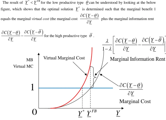
^FB

The result of

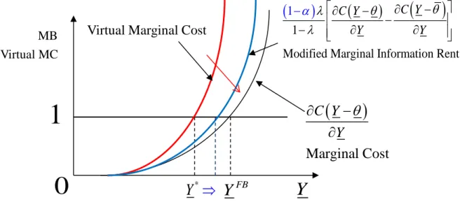
Y

^*

< Y

^FBfor the low productive type

θ

can be understood by looking at the below figure, which shows that the optimal solution

Y

^* is determined such that the marginal benefit 1 equals the marginal virtual cost (the marginal cost

^{C Y} ( )

Y θ

∂ −

∂

plus the marginal information rent

( ) ^{C Y} ( )

C Y

Y Y

θ ^∂ ⁻ θ

∂ −

∂ − ∂

for the high productive type

θ

.

Figure 1: Optimal Solution

Y

^*for Low Productivity Type

θ

The Concept of “Bao 包 (Contract)”

The concept of “Bao” 包 (Contract) can be understood better by exploring the optimal fiscal incentive contract between the Central and Local governments.

7 This is a familiar result in the literature (e.g. Baron and Myerson (1982), Maskin and Riley (1984), and Bolton and Whinston (2005)).

MB Virtual MC

Y

*

^Y

0

1 ⁽ ⁾

Marginal Cost C Y

Y

∂ − θ

∂

( ) ( )

1 Marginal Information Rent C Y C Y

Y Y

θ θ λ

λ

 ∂ − ∂ − 

−

 

−   ∂ ∂  

Y

FB

Virtual Marginal Cost

(14)

12

First, by differentiating both sides of

^T ^{= −} ^Y ^{C Y} ( ⁻ ^θ ) ⁻ { ^{C Y} ⁽ ⁻ ^θ ⁾ ⁻ ^{C Y} ( ⁻ ^θ ) }

^by

^Y

^{, and}

combining the first order condition (8), we have^{T Y}^′

( )

^FB ^{= −}¹ ^{C Y}^′

(

^FB⁻

^θ )

⁼⁰, which means that regarding Local governments of the high productive type (abundant regions), the marginal Tax paid to the Central government according to the marginal growth of GDP is zero at the optimum. It follows that¹⁻^{T Y}^′

( )

^FB ⁼¹, which means that 100% of the marginal rate of the remainder of the local fiscal revenue belongs to the Local government of the high productive type (abundant regions).⁸ That is, the high productive type

θ

can receive 100% of the marginal benefit from GDP growth. This, in essence, is the same as the “100% piece-rate system”.⁹

Next, by differentiating both sides of

^T ^{= −} ^Y ^{C Y} ( ⁻ ^θ )

^by^Y and combining the first order condition (9), we have

^{T Y} ^′ ( ) ^{= −} ¹ ^{C Y} ^′ ( ⁻ ^θ ) ⁼ ( ) ( ) ( )

1 λ C Y θ C Y θ

λ ^ ^ ^′ ⁻ ⁻ ^′ ⁻ ^ ^

−

( ) ⁰

T Y ′ >

means that regarding the low productive type

θ

, the marginal Tax paid to the Central government according to the marginal growth of GDP is positive. That is, Local governments cannot receive 100% of the marginal benefit of GDP growth, i.e.,

¹ ⁻ ^{T Y} ^′ ( ) ^< ¹

^and

^{T Y} ^′ ( )

flows to the Central government. Therefore, the marginal incentive also decreases

Y

^*

≤ Y

^FB at the optimum.

In summary, we have

Proposition2 The degree of “Bao” 包 (Contract)

^b ( ) ^θ

can be understood as the marginal rate of the local fiscal revenue. It increases in the productivity type θat the optimum, as follows.

( ) ( ( ) ) ( )

*

1 ( ) 1 for

1 1 1 for

T Y

FB

b T Y

T Y

θ θ θ θ

θ θ

*

 − ′ = =

′ 

= − = 

− ′ < =



The theoretical intuition behind this proposition is as follows. To maximize the expected total surplus (efficiency), the Central government should set the GDP for the low productivity region

θ

8 The concept of “Bao” 包 works similarly in the “Household contract responsibility” system, which began in rural areas in 1978. The system introduced market incentives to agricultural production and resulted in a dramatic increase in agricultural productivity. See, McMillan, J. (1992) and McMillan, J. et al. (1989).

9 Jin, Qian, and Weingast (2005) found a high marginal piece-rate value of 0.8~0.9 in 1989-1993 (later

“Fiscal contracting” period).

(15)

13

at the first best level

Y

^*

= Y

^FB. However, the Central government must then give up the larger information rent for the high productive type

θ

. As an optimal solution to the trade-off between the GDP for the low productivity region

θ

and the information rent for the high productive region

θ

^,

the Central government induces the lower GDP

Y

^*

< Y

^FB for the low productivity region

θ

^,

which is a second-order loss, but attains the Tax increase through reducing the information rent for the high productive region

θ

, which is a first-order gain. To induce the lower GDP

Y

^*

< Y

^FB^{, the}

Central government adopts a less-than 100% “Bao” (Contract)

^b ( ) ^θ ^< ¹

, that is, a lower-powered incentive scheme for the low productivity local government

θ

.¹⁰

2.3.2 Graphical Explanation

The objective function of the Local government (agent of type

θ

) is

^{U Y T} ( ^{, :} ^θ ) ^{= − −} ^Y ^T ^{C Y} ( ⁻ ^θ )

and this draws an indifference curve of type

θ

on the

( ^{Y T} ^, )

^plane.

We obtain a marginal rate of substitution for type

θ ( )

const.

YT

1

U

MRS dT C Y

dY

θ

=

= = − ′ −

.

The first order condition for the optimality which characterizes the first best solution is

( )

1 − C Y ′ − θ = 0

, from which we defineY− =

θ

e^FB. This then proves that at the first best solution, the effort levels of each type are equal

e

^FB

= e

^FB

= e

^FB, and since

Y

^FB

− Y

^FB

= − θ θ

, the difference in GDP level is only the difference in the productive type. In this case, as

( )

0 1 0

0

FB FB YT

FB

if Y e

MRS C Y if Y e

if Y e

θ

θ θ

θ

> < +

 

= − ′ −  = = +

< > +



shows, the indifference curve of each type

θ

reaches its peak at the first best GDP level

10 This argument is based on the (standard) assumption that the Central government maximizes only its own expected payoff and does not put any weight on the Local governments’ payoffs. In the appendix, we examine the optimal solution when the Central Government is altruistic and puts a positive weight on the high productivity type’s payoff.

(16)

14

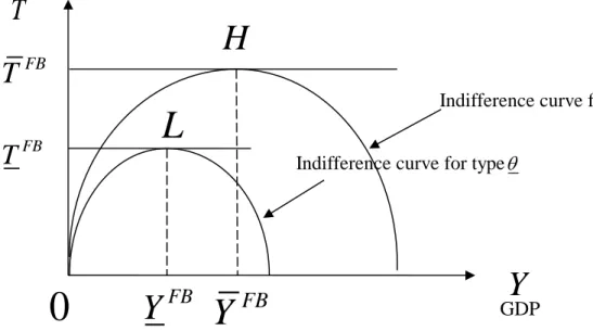
FB FB

Y = +

θ

e and becomes an upward-convex symmetric parabola (see diagram below). The first best solutions are L and H in the diagram.

Figure 2: Indifference Curves and First Best Solutions for both types

θ

and

θ

Under perfect information, the Central government is able to identify type information, such that it can assign and enforce the pointL in the diagram to type

θ

and the pointHto type

θ

^.

However, under asymmetric information as in the diagram below, the gain will be higher by

( )

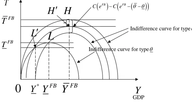
^FB

(

^FB

( ) )

C e − C e − θ θ −

if the high productive type

θ

chooses pointLinstead of pointH, and this produces an incentive to disguise its information as being the low productive type

θ

.

Figure 3: Incentive for high productive type

θ

to choose pointL FB

L

T T

FB

H

0 _Y ^FB _Y ^FB

T

GDP Y

( )

^FB

(

^FB

( ) )

C e −C e −

θ θ

−

GDP Y

T

Y FB Y ^FB

0

FB

H

T

FB

L Indifference curve for type θ

Indifference curve for typeθ

(17)

15

This will result in lowering the tax revenue of the Central government (

T

^FB

− T

^FB

= − θ θ

).

Therefore, the Central government gives up the first best solution, offers the two contract menus

{ ^{L H} ^{′ ′} ^, }

as shown below, elicits true information by inducing type

θ

to choose L′, and type

θ

to choose H′, and achieves a payoff increase.

Figure 4: Second Best Solutions H′ and L′

At pointH′_{, because}^{T Y}^′

( )

^FB ⁼⁰, the rate to be paid to the Central government according to the marginal growth of the regional GDP is zero, and with ¹⁻^{T Y}^′

( )

^FB ⁼¹being virtually the same as a “100% piece-rate system,” 100% of the marginal GDP growth belongs to the Local government.

Therefore, an incentive for the first best solution is derived (“Efficiency at Top”).

Conversely, because^{T Y}^′

( )

^* ^>⁰, Local governments cannot receive 100% of the marginal result of GDP growth at pointL′, and the portion

^{T Y} ^′ ( )

^* flows to the Central government. Thus, the derived marginal incentive also decreases (“Downward Distortion at Bottom”).

GDP Y

T

Y FB Y ^FB

0

FB

H

T

FB

L

( )

^FB

(

^FB

( ) )

C e −C e −

θ θ

−

H ′

L ′ Indifference curve for typeθ

Indifference curve for typeθ

Y

*

(18)

16

3 ． Competition between Local Governments: the Yardstick Mechanism in Correlated Environments

The Concept of “Bisai 比賽 (Contest)”

It is also said that “Bao 包(Contract)” and “Bisai 比賽 (Competition)” function in combination within the relation between the Central and Local governments as an institutional basis of the Chinese economy after “reform and opening-up.” Now, 比賽 (Competition) will be analyzed within the framework of the yardstick competition between the Local governments to show the information disclosure function through comparison and competition.

In the case where productivity information is “perfectly correlated”¹¹ between two regions, truth-telling (honest revelation of productivity) can be achieved as a dominant strategy equilibrium by generating a “Prisoner’s Dilemma” game of information revelation. In equilibrium, there is no need to give informational rent to the Local government, and the first best solution can be achieved.

Even when the situation is not in perfect correlation but is close to it, informational rent could be decreased and efficiency increased, compared with the case without comparison and competition.

The private information

( ^{θ θ}

ⁱ^, ^j

)

of Local governments

i j ,

are perfectly correlated, i.e.

( ^, ) ( ) _{( )} ^, ^{with prob.}

with prob. 1

i j

,

θ θ λ

θ θ θ θ λ

=    −

(

^,

) ⁽ ⁾

i i i j i i

Y −T Y Y −C Y −

θ

is the payoff function of Local government i in the case where the

Local government i_(type

θ

_i) achieves

Y

_i(GDP), and Local government

j

(type

θ

_j) achieves

Yj(GDP).^{T Y Y}

(

ⁱ^, ^j

)

is the tax amount paid to the Central government (Taxation). Hence, we can regard ^{T Y Y}

(

ⁱ^, ^j

)

as a “Fiscal contract” proposed by the Central government.¹²

11 We can generalize it to a more general setting, including imperfect correlation. Although a possible framework would be an optimal auction model, it seems to be rather difficult for the Central government (the State) to design the elaborate optimal auction-type mechanism ex ante and commit to it. In other words, some contract incompleteness would accompany the concept of “Bisai” (Contest) and its mechanism.

12 We describe the relationship between the central and local governments by the contract theory framework that assumes players are independent entities, according to the “Local State Corporatism” of Oi (1992), rather than by a hierarchical relationship in an organization.

(19)

17

( )

( ) ( ) ( )

( ) ( ) ( ( ) ) ( ) ( )

( )

FB total surplus for type

FB total

Information Rent

s

Δ

u

if , ,

,

FB FB FB FB

i j

FB FB FB FB

i j

FB FB FB FB

i j i i j

FB F

FB B

B

F

e C e Y Y Y Y

T Y Y

e C e

C e C e

θ

θ θ

θ

+ − =

=

+

 

− − − − + ∆

−

 

 ((((  ((((( ((((( ( (

＋

( ) ( ( ) ) ( ) ( )

Information Rent

rplus for type Δ

if , ^FB,

FB B B

j

F F

C e C e Y Yi Y Y

θ

θ θ









  =

 + − − − + ∆

(((( ((((((((((((

＋

The point of this scheme is the side transfer (payoff transfer) from the Local government with a low GDP

Y

^FB(

θ

reported) to the Local government with a high GDP

Y

^FB(

θ

reported). This scheme incorporates the payoff change, the term Δ, due to the promotion/demotion of the local executives (officials) based on the relative outcome of the regional growth (GDP) competition. As a whole, therefore, we can interpret the model of this section as a contest model to incorporate the incentive effect of yardstick competitions.¹³

First, we explore the incentive of the local government of type

θ θ

_i = in the state

( ) ^{θ θ}

^, ^under

the above scheme. His payoff function is written as^Yⁱ⁻^{T Y Y}ⁱ

(

ⁱ^, ^j

) (

⁻^{C Y}ⁱ⁻

^θ )

, which is the payoff when the Local government of type

θ θ

_i = chooses the output (GDP)

Y

_i given that the other

Local government chooses the output (GDP)Y_j.

*Suppose that the other Local government

θ

_j

= θ

chooses the low outputY^FB.

Then, if the Local government

θ θ

_i = chooses the low outputY^FB, he will obtain the payoff

( ^, ) ( ) ( ) ( ( ) )

FB FB FB FB FB FB

Y − T Y

i

Y − C Y − θ = C e − C e − θ θ −

_.

If the Local government

θ θ

_i = chooses the high outputY^FB, he will obtain the payoff

13 Li and Zhou (2005) empirically show that in China, the government official promotion process resembles a tournament, and the final decision is mainly based on relative performance in economic growth. The contest model of this section would be suitable for such situations.

(20)

18

( ) ( )

( ) ( ) ( ( ) )

{ } ^{( )}

FB FB

,

FB FB

i

FB FB FB FB FB FB

Y T Y Y C Y

e e C e C e C e C e

θ

θ θ θ θ

− − −

 

= + − + − −  − − − + ∆  −

( )

^FB

(

^FB

( ) )

C e C e θ θ

= − − − + ∆

.

Hence, the Local government

θ θ

_i = has an incentive to choose the high output (GDP)Y^FB.

*Next, suppose that the other Local government

θ

_j

= θ

chooses the high output (GDP)Y^FB.

θ θ

_i = chooses the low output (GDP)Y^FB, he will obtain the payoff

( ) ( )

( ) ( ) ( ( ) )

{ } ⁽ ⁽ ⁾ ⁾

FB FB

,

FB FB

i

FB FB FB FB FB FB

Y T Y Y C Y

e e C e C e C e C e

θ

θ θ θ θ θ θ

− − −

 

= + − + − +  − − − + ∆ −  − −

= −∆

θ θ

_i = chooses the high output (GDP)Y^FB, he will obtain the payoff

(

^,

) ( )

⁰

FB FB FB FB

Y −T Yi Y −C Y −

θ

= ^.

θ θ

_i = has an incentive to choose the high outputY^FB. That is,

regardless of the other player

θ

_j

= θ

’s choices, the Local government

θ θ

_i = has a strict incentive

to choose the high outputY^FB.

The incentive structure of the Local government

θ

_j

= θ

is also the same. Regardless of the

other player

θ θ

_i = ’s choices, the Local government

θ

_j

= θ

has a strict incentive to choose the

high outputY^FB. The choice of Y^FB is the dominant strategy for the agent

θ

_j

= θ

. The payoff matrix is as follows.

Note that perfect correlation of the private information

( ^{θ θ}

ⁱ^, ^j

) ( )

⁼

^{θ θ}

^, can be relaxed.

Essentially, as the payoff matrix shows, the Central government places the two Local governments in a prisoner’s dilemma game. By exploiting this structure, the Central government can implement the

(21)

19

full information first best optimum in the unique dominant strategy equilibrium.¹⁴

θ

j

= θ

θ θ

i = Y^FB Y^FB

^{C e} ( )

^FB

⁻ ^{C e} (

^FB

⁻ ( ^{θ θ} ⁻ ) )

^{C e} ( )

^FB

⁻ ^{C e} (

^FB

⁻ ( ^{θ θ} ⁻ ) ) ^{+ ∆}

Y^FB

^{C e} ( )

^FB

⁻ ^{C e} (

^FB

⁻ ( ^{θ θ} ⁻ ) )

−∆

−∆ 0 Y^FB

^{C e} ( )

^FB

⁻ ^{C e} (

^FB

⁻ ( ^{θ θ} ⁻ ) ) ^{+ ∆}

0

Table 3: Incentive Structure for High Productivity Types

( ) ^{θ θ}

^,

Next, we explore the incentive of the agent of type

θ θ

_i

=

in the state

( ) ^{θ θ} ^,

. His payoff function is written as ^Yⁱ⁻^{T Y Y}ⁱ

(

ⁱ^, ^j

)

⁻^{C Y}

⁽

ⁱ⁻

^θ ⁾

when the Local government

θ θ

_i

=

chooses the output (GDP)

Y

_i given that the other Local government chooses the output (GDP)Y_j.

*Suppose that the other Local government

θ

_j =

θ

chooses the low outputY^FB.

θ θ

_i

=

chooses the low outputY^FB, he will obtain the payoff

( ^, ) ( ) ( ) ( ) ⁰

FB FB FB FB FB FB FB FB

Y − T Y

i

Y − C Y − θ = + θ e −   θ + e − C e   − C e =

^.

θ θ

_i

=

chooses the high outputY^FB, he will obtain the payoff

14 A key problem in the design of optimal contracts in correlated environments is the possibility of multiple equilibria in the subgame played by the parties whose private information is correlated. As noted by Demski and Sappington (1984), multiple equilibria do not pose a problem when the private

information is perfectly correlated. Shleifer (1985) presents a theory of Yardstick Competition in the perfect correlation environment in the regulation context.

(22)

20

( ) ( )

( ) ( ) ( ( ) )

{ } ⁽ ⁽ ⁾ ⁾

( ) ( ) ( ( ) ) ( ( ) )

FB FB

,

FB FB

i

FB FB FB FB FB FB

FB FB FB FB

Y T Y Y C Y

e e C e C e C e C e

C e C e C e C e

θ

θ θ θ θ θ θ

θ θ θ θ

− − −

 

= + − + − −  − − − + ∆ −  + −

 

= +  − − − + ∆ −  + −

( ) ( ⁽ ⁾ ) ( ⁽ ⁾ )

2 2

FB FB

FB

C e C e

C e θ θ θ θ

−

 − − + + − 

 

= −

 

 

+ ∆

((((((((((((((((((

The negative sign is due to the convexity of the cost functionC′>0,C′′>0.

θ θ

_i

=

has an incentive to choose the low output (GDP) Y^FB if ∆ is sufficiently small.

Fiscal Relations between the Central and Local Governments in China and the Concepts of "Bao (Contract)" and "Bisai (Contest)" : A Contract Theory Analysis