The backward-bending commute times of married women with household responsibility
Shinichiro Iwata
Faculty of Economics, University of Toyama 3190 Gofuku, Toyama 930-8555, Japan
Keiko Tamada
Faculty of Economics, Fukuoka University
Nanakuma 8-19-1, Johnan-ku, Fukuoka 814-0180, Japan [email protected]
Abstract
The purpose of this paper is to examine theoretically and empirically whether the com- mute times of married women follow a backward-bending pattern with respect to wage rates.
The existing literature has shown that married women tend to choose short commutes be- cause of their relatively low wages combined with comparatively heavy household responsi- bilities. However, a work–leisure model, which includes the simultaneous decision wives take regarding commute times and wage rates, suggests that married women employed in highly paid positions also undertake short commutes, while married women with wage rates in the middle range choose long commutes. These results suggest that the commute times of mar- ried women display a backward-bending pattern. Applying an instrumental variable strategy that accounts for the endogeneity of wage rates, the empirical results for employed married women in Japan appear to support this …nding. Moreover, one of our results suggests that highly paid married women can still secure greater leisure time with short commutes, despite retaining a heavy load of domestic responsibilities.
Keywords Commute times; leisure time; household responsibilities; married women
1 Introduction
In most countries, domestic chores remain the primary responsibility of many married women, even though they are often also in full-time employment.1 As a result, household responsibilities can be seen as a constraint on the personal leisure time of married women. In these circum- stances, how do married women working full time secure leisure time?2 Two broad strategies are possible. The …rst is a reduction in working hours. In general, employed women may work longer when their wages increase. However, as wages increase further, they may reduce their working hours in order to set aside time for leisure. Of course, the backward-bending supply curve of labour is well known from standard economics texts.3 Instead, we focus on a second strategy that tends to be e¤ective, especially when the …rst strategy is commonly impracticable.
That is, women may reduce their travel time to work to increase the time available for leisure.
In this situation, does a backward-bending relationship also arise between commute time and wage rates? The major objective of this paper is then to o¤er both theoretical and empirical evidence on how married women who share household responsibilities change their commute times in response to changes in wage rates.
A number of early studies suggested that married women have a tendency to travel long hours for work in tandem with the increase in wage rates (e.g., Singell and Lilllydahl 1986; Pazy et al. 1996). A few recent analyses, however, have demonstrated that married women with high wage levels appear to commute for short periods in order to secure additional time to spend on domestic chores, parenting, and leisure (e.g., Freedman and Kern 1997; Prashker et al. 2008).
Connecting these suggestions invokes a novel hypothesis: the backward-bending commute times of married women with household responsibilities at high wage rates. To our knowledge, this paper is the …rst to examine this particular hypothesis.
We develop a theoretical model of dual-income households that choose the household’s res-
1Using the Harmonised European Time Use Survey (HETUS, online database Version 2.0.), we can obtain evidence on the contribution rate of married men to total housework hours in dual-income households for persons aged 20–74 years with both spouses working full time. This clearly suggests that married men in European countries have relatively fewer household responsibilities: 38.1% in Belgium, 31.8% in Bulgaria, 35.4% in Estonia, 38.3% in Finland, 37.4% in France, 42.5% in Germany, 27.4% in Italy, 32.3% in Latvia, 30.8% in Lithuania, 39.2% in Norway, 36.5% in Poland, 35.0% in Slovenia, 33.6% in Spain, 41.9% in Sweden, and 40.1% in the United Kingdom. Married men in Japan bear even less of the share of domestic responsibilities with the 2006 Survey on Time Use and Leisure Activities (STULA, Statistics Bureau, Ministry of Internal A¤airs and Communications) informing us that the contribution rate of married men to total housework hours in dual-income households for persons aged 15 years or older is only 10.4%.
2Women may also lose opportunities to participate in activities because of household responsibilities. We, however, do not consider this issue.
3Married women may also alter the days on which they work during the week. We do not consider this possibility here, however, because we focus on how married women divide their time use during the working day.
idential location and the wife’s workplace. We assume that di¤erent workplaces yield di¤erent levels of female wage rates. When dual-income households determine homes and workplaces, the commute times of married women are simultaneously determined. A comparative static analysis of this model then informs us about the relationship between the commute times of wives and their wage rates. To consider the simultaneous decision regarding commute times and wage rates, we apply an instrumental variables (IV) approach. Our data set, which employs the Japanese Panel Survey of Consumers conducted by the Institute for Research on Household Eco- nomics, permits us to estimate this relationship. Using the sample of working wives, we regress commute times on monthly wage rates and the square of monthly wage rates. At the same time, we address the simultaneity of female wage rates by estimating female wage rates controlled by a proxy variable for the workplace. Our hypothesis infers that the estimated coe¢ cient for wage rates will be positive while that for its square will be negative.
In accordance with changing commute times, married women potentially allocate their time available across housework and leisure. Both our theoretical and empirical model incorporate these accompanying issues. In the estimation stage, both housework and leisure times are estimated using the same procedures detailed above. Therefore, married women non-linearly allocate their time use through the wage.
The remainder of the paper is organized as follows. Section 2 provides a review of the relevant literature. In Section 3, we present the theoretical model of married women’s behaviour. Section 4 discusses the data and empirical model along with the empirical results and Section 5 o¤ers some suggestions for future research. Finally, Section 6 summarizes the main conclusions of the analysis.
2 Literature review
2.1 Economics approach
Kain (1962) empirically demonstrated that females tend to make shorter journeys to work than their husbands.4 Kain (1962) suggested that working married women with household respon- sibilities are e¤ectively secondary wage earners and consequently they are more likely to seek
4Again using the HETUS, we estimate that the commute times (in minutes, for persons aged 20–74 years in full- or part-time work) for married women (men) are 25(37) in Belgium, 38(46) in Bulgaria, 35(38) in Estonia, 23(28) in Finland, 28(40) in France, 23(39) in Germany, 34(47) in Italy, 38(50) in Latvia, 38(44) in Lithuania, 24(34) in Norway, 34(43) in Poland, 28(32) in Slovenia, 38(45) in Spain, 23(28) in Sweden, and 25(41) in the United Kingdom. Japan displays similar features. According to the STULA, the commute times in Japan (in dual-income households for persons aged 15 years or older) are 27 minutes for women and 47 minutes for men.
convenient positions of employment near the home. Various approaches, such as economics, sociology, transportation, women’s studies, and others have demonstrated a variety of empir- ical results that are consistent with Kain’s (1962) argument. In this section, we …rst review the literature based on an economics approach. However, we also review several studies under- taken in other …elds that also support the economics approach. We then review the relevant transportation literature.
With regard to household responsibilities, Johnston-Anumonwo (1992) and Turner and Niemeier (1997) found that commute times for women appears more sensitive to marital status;
Turner and Niemeier (1997) and Lee and McDonald (2003) demonstrated that the presence of children tended to reduce women’s travel time to work; and Freedman and Kern (1997) concluded that married women, especially those who have children, are less likely to choose a workplace and/or residential location where the commute times are longer. In general, these studies indi- cate that women choose shorter commutes when faced with greater household responsibilities.
In other work, Hanson and Johnston (1985) found that female-dominated employment op- portunities are distributed relatively uniformly within cities. In general, women also obtain lower wages than men. Accordingly, if there is less spatial variation in women’s wages at low wage levels, women have less of a reason to commute and their work trips are commensurately shorter. Therefore, as suggested by Madden (1981), it is not rational for married women to perform long commutes to obtain low wages.
Economists have subsequently formulated a theoretical location model that attempts to capture Kain’s (1962) essential argument. White (1977), for example, argued that couples determine residential locations together given the husband’s employment opportunities in the city centre and those of the wife in the suburbs. Both the husband’s and the wife’s time and budget constraints are incorporated in this model. The model suggests that dual-income households choose their residential locations so that the wife’s commuting journey is shorter than that of the husband’s, namely, they reside nearer the suburban job where housing prices are relatively lower. Later, White (1986) suggested that female household heads may prefer a shorter commute because their tastes di¤er from those of male household heads. That is, the market wages of females are unable to be su¢ ciently high to induce them to commute more than a minimum distance because of their heavy responsibilities at home. Madden (1981) and Singell and Lillydahl (1986) empirically supported White’s (1977) views by …nding that families select a suburban residence to accommodate the housing demands associated with raising children. In
this situation, working females have reduced commute times because of their existing household responsibilities and the relative concentration of female employment in the suburbs.
In sum, geographically smaller female-dominated labour markets with relatively lower earn- ings and the traditionally greater share of household responsibilities held by wives imply shorter work-related journeys for married women. Much of the existing research has been mostly ap- plicable to part-time workers because they are usually employed in female-dominated positions with low wages. However, the number of females employed as full-time workers in traditionally male-dominated positions earning higher wages has continued to increase. Indeed the growing involvement of women in the paid labour force has raised signi…cant questions about transporta- tion (Zhang et al. 2012). To stimulate research on this issue, four conferences on women’s issues in transportation were held by the Transportation Research Board in 1978, 1996, 2004, and 2009. In general, full-time female workers are more likely to encounter greater spatial varia- tion in wages than part-time workers. In this regard, Madden (1981), followed by Madden and Chen Chiu (1990) and Freedman and Kern (1997), developed location models where dual-income households jointly select the household’s residential location and the husband’s and wife’s work- places. This assumption allows married women with middle- or high-range wages to partake in long journeys for work. Singell and Lillydahl (1986), Pazy et al. (1996), Turner and Niemeier (1997), and Lee and McDonald (2003) empirically found that female wages (or proxies for fe- male wages) have a positive impact on commute times for wives. Somewhat surprisingly, Plaut (2006) showed that commuting distances for women are equally or even more sensitive to income increments than are those of men. As suggested by Madden (1981), Singell and Lillydahl (1986), Pazy et al. (1996), and Lee and McDonald (2003), the question is then whether married women earning middle- or high-range wages travel for longer times to work much like their husbands.5 Some recent studies have reported divergent responses to this question. For instance, Sandow and Westin (2010) addressed the duration of long-distance commuting (45 minutes or longer to work, one way), and found that women are more likely to give up long-distance commuting because of their household responsibilities. Elsewhere, Freedman and Kern (1997) and Mok (2007) concluded that the location decisions of dual-income households are more sensitive to the earnings of wives than husbands. These results di¤er markedly to those in early studies, in- cluding Madden (1981) and Singell and Lillydahl (1986), which appear to show that the choice
5The reason for long-distance commuting is not solely wage-related. Married women tend to choose long commutes when they can develop coping strategies for managing their mobile life; they can get support from their spouse; they want to maintain local ties in suburbs, especially for their children (Hofmeister 2005; Sandow 2011).
of residential selection is more heavily in‡uenced by the job location of husbands given that their earnings generally exceed those of their wives. On this basis, Freedman and Kern (1997) predicted that highly educated wives working full time in a professional career to a large ex- tent favour a city location, even though they could choose a suburban home, because they …nd the commuting involved burdensome. Another result in Prashker et al. (2008) indicated that women earning at the highest income levels tend to relocate their residence more than men when their commute becomes relatively longer. They suggested that this might re‡ect the fact that cultural standards impose constraints on women with respect to handling household responsi- bilities, and thus women with higher income levels are willing to pay a high price for living close to work. On the other hand, several studies have suggested that full-time working mothers appear to feel guilt over their inability to ful…l specialized housework duties, such as child-care (Hofmeister 2005; Kim and Ling 2001; Lee 2002). Recent studies have also demonstrated that commuters with longer travel times are more likely to feel stress than commuters with shorter times (Hofmeister 2005; Sandow 2011). Roberts et al. (2011) indicated that commuting has an important detrimental e¤ect on the well-being of women, but not men. They suggested that women’s greater sensitivity to commuting time seems to be a result of their greater responsibil- ity in the household. In this regard, married women may attempt to spend more time on child rearing and household chores as wages increase by living closer to their workplace.
As discussed, the literature has long assumed that the choice of residential location is gener- ally based on either the husband’s employment site or other factors such as the price of housing, the distance to the nearest railway station, or the quality (atmosphere) of the residential area.
Therefore, the extent of women’s rights in deciding their residential location appears a contro- versial issue. In Japan, however, the results of several recent studies based on Kitamura’s (2010) report may be applicable to our theory. Kitamura (2010) found that dual-income households with children who have experienced job transfers prefer to locate their residence close to the wife’s employment site rather than that of the husband. Kitamura (2010) used this to sug- gest that this household strategy may help mitigate the heavy burden of household duties and child-care placed on working mothers.
Connecting these arguments motivates us to analyse whether the relationship between the commute times of wives and their wages follows a backward-bending pattern in relation to household responsibilities. To explore this relationship, we examine middle-range and highly paid wives working full time. Although we do not directly examine the extent of women’s rights
to decide their residential location, we believe that this relationship indirectly provides this information.
Our selected approach is clearly economic. Similar to Madden (1981), Madden and Chen Chiu (1990), and Freedman and Kern (1997), we develop a theoretical model because the compar- ative statics provide insights into what conditions and how women’s wages alter their commute times. The theoretical model is also meaningful when interpreting the signs of the estimated coe¢ cients. Because we do not assume any speci…c form of utility function, we arbitrarily chose our empirical speci…cation to examine this theoretical hypothesis. The literature has frequently estimated a linear form of commute time function, while some studies have applied quadratic functions because of the assumption that the structure of household preferences is twice con- tinuously di¤erentiable. In this analysis, we carry the wage rate variables in the commute time equation up to the quadratic term to consider our hypothesis. We also attempt to overcome and simultaneity bias in that women in our model can theoretically choose their wage rate, thereby indicating that increases in commute times are likely to induce employers to o¤er higher wage rates. Indeed, Sandow and Westin (2010) tested this reverse causality. Therefore, as in Madden (1981) and Singell and Lillydahl (1986), we employ IV regression to take into account the simultaneity arising with wage rates.
2.2 Economics of time use
If married women increase the time spent commuting as wages rise, they may have to sacri…ce their leisure time relatively more than their husbands because of their comparatively heavier household responsibilities. In fact, Fuess (2012) found that Japanese females spend fewer hours on weekday leisure activities than males. Therefore, reducing commute times tends to be a strategy for working women to increase the time spent on leisure. Inspired by the seminal ideas of Gary Becker (1965), economists have generally assumed that people receive utility from time engaged in leisure, not market and household work. Household work includes the time an individual spends on household production activities such as cooking, laundry, and house, car, lawn, and garden maintenance; child-care and care of the sick; and planning, shopping, and other family managerial activities, whereas leisure time is de…ned as the time not spent in market or household work (Bryant and Zick 2006). Therefore, to improve the well-being of married women, it may be important to better understand how married women secure leisure time by making adjustments in their use of other time. To do this, Solberg and Wong (1992)
constructed a theoretical model of the household where the time use of each person is divided into market work, home production, leisure, and work-related travel time. However, they consider that the latter is predetermined. They then estimated the time-use equations controlled by quadratic forms of the explanatory variables. Their empirical results suggest that travel time to work reduces the wife’s leisure and housework times at an increasing rate. The urban economic literature associated with the shorter commute times of married women, however, has received little attention in terms of the time spent on their leisure. The literature has also generally considered that the time spent on housework is a given. In this regard, this analysis considers how married women divide their time use into leisure as well as household production as a secondary issue. In doing so, we pay close attention to the relationship between time use and wage rates. This is because the opportunity cost of the time spent on housework and leisure is generally captured by wage rates; that is, if people surrender housework and leisure time, they can work and earn more income.
2.3 Transportation approach
Female activity–travel patterns are quite complex analyses because household responsibilities frequently generate additional constraints on daily schedules. Unlike economists, transportation researchers have tended to focus on how travel time and household responsibilities in‡uence the time spent on leisure activities using activity-based models. The understanding of leisure activities, especially those performed outside the home, then appears to be important because they increase the demand for travel from the home to a speci…c activity destination, which is usually di¢ cult to forecast in practice.
Kitamura et al. (1996) found that individuals with longer commutes are less likely to pursue out-of-home discretionary activities. Their empirical results also suggest that women with chil- dren tend to be less oriented towards these out-of-home discretionary activities. Meloni et al.
(2009) demonstrated that women who have longer work trips devote less time to participating in out-of-home recreation and leisure. As an alternative, Zhang et al. (2012) focused on the in‡uence of child-care on the time allocation of women. Commute time, however, was included in market work time. Their empirical results con…rmed that having a child reduces time use for leisure and labour and increases housework time. The level of education for women, which may proxy for their wages, exerts a similar in‡uence on time use.
In the activity-based behaviour model, all time variables, such as housekeeping and com-
muting, are entered to the utility function as arguments. The literature has also tended to focus on corner solutions, that is, the decision to participate in an activity. For example, Kitamura et al. (1996) and Meloni et al. (2009) developed a model where single households choose which activities to participate in and how much time to allocate among various activities, while Srini- vasan and Bhat (2005) and Zhang et al. (2005, 2009, 2012) extended the model to encompass decisions jointly made by multiple persons incorporating intra-household interaction. Generally, a speci…c form of utility function is assumed, because it provides a speci…c form to be estimated, with modi…ed probit, logit, and Tobit models formulated using their theoretical model.
As discussed, a growing literature in the transportation approach has considered the cause- and-e¤ect relationships between commute times, household responsibilities, and the wage rates of females. Nonetheless, the attention paid to the non-linear relationship between female commute times and wage rates with household responsibilities has been limited. We thus believe that the present analysis may serve to complement the …ndings in these earlier studies.
3 The model of married women
3.1 The model speci…cation
The main purpose of this section is to obtain the relationship between wage rates and the commute time of married women living with their husbands. We start with a brief outline of the model. Further details of the model follow the outline.
3.1.1 The outline of the model
There are three options available in the women’s work–home location choice, all of which include di¤erent combinations of the female wage rate, the commute times of both a married woman and her husband, and their cost of living.
Under each option where the combination of the wage rate, the commute times of the each spouse, and living cost are given, the married woman and her husband …rst seek the optimal levels of their housework, market work, and leisure times that maximize the household’s utility level subject to their budget and time constraints.
The married couple then selects the combination of the wage rate, commute times, and living cost that generates the highest utility from the three options.
3.1.2 The three options
Now let us introduce the several combinations of work–home location. Suppose that there are two workplaces available for the wife that are located in the city centre and a suburb. For simplicity, her husband’s workplace is …xed in the city centre. Her wage rate is wF in the suburb and wF in the city centre, where F indicates female. We assume that wF < wF. The living cost, for example, the rental costs of housing in the suburb, is written asr, which is lower than the living cost in the city centre,r: r < r. We assume that the married couple consumes a single unit of housing throughout the analysis.6
The couple is assumed to have three options available, as in Fig. 1. The …rst (and benchmark) option is that she may work and reside in the suburb, where her commute time is denoted by c. Her husband’s commute time is written as cand assumed to be c < c, because the husband is assumed to commute to the city centre from the suburb. Therefore, the benchmark option is similar to the theoretical model in White (1977). In brief, White (1977) suggested that married men residing in a suburb with their wives are more likely to work in the central city and commute for longer hours, whereas their wives are more likely to work in the suburban ring and commute for shorter hours.
The second option is that the married woman may work in the city centre while continuing to reside in the suburb, but commuting regularly to work. The married woman then becomes a long-time commuter (c) under this option because she works and resides in di¤erent areas.
Under this option, her husband continues to make a long commute to work.
The third option is that the married woman may both work and reside in the city centre.
She then becomes a short-time commuter (c) because she again works and resides in the same area. Under this option, her husband also becomes a short-time commuter because the married couple selects a residence close to the husband’s workplace, which is also located in the city centre.
3.1.3 First stage: decisions on time use under each option
In the …rst stage, the married couple solves a constrained maximization problem for each option discussed above. Thus, we next consider the utility maximization problem of the j-th option (j = 1;2;3). A formal model of the time allocation of households in the manner of Gronau
6Relationships between the commuting decisions of spouses in dual-income households and their housing pref- erences were studied, for example, by Singell and Lillydahl (1986) and Plaut (2006).
(1977) is presented. Gronau (1977) assumed that the time use for each person is divided into three basic activities: market work, home production, and leisure. In this analysis, however, these basic activities are extended to include the time spent on commuting, as in Solberg and Wong (1992). Note that the commute times for both the wife and the husband are given at this stage.
LetM denote the male,lkj denote the leisure time ofk(k=F; M), andxj a composite good.
Under thej-th option, given the wage rate, commute time, and living costs, the married woman and her husband are considered to maximize the following additive utility function:
j =uF(lFj ) +uM(lMj ) +g(xj); (1) where uk( ) and g( ) are the sub-utility functions. Both uk( ) and g( ) exhibit positive and diminishing marginal utilities: ukl > 0, ukll <0,gx >0, gxx <0, where subscripts indicate the
…rst and second derivatives.
The quantity ofxj consumed by the household is given by the sum of goods purchased in the market and the goods produced at home (Gronau 1977; Solberg and Wong 1992). The quantity of market goods is then given by:
xmj =wFj mFj +wMmMj +IF +IM rj;
wheremkj is the working time in the market, Ik is the sum of non-labour income, and rj is the living cost. Non-labour income Ik is assumed given. Because we shed light on the monetary value assigned to time saving in commuting, the pecuniary commuting cost is assumed to be zero. This helps simplify the model. To recount, the living costsrj and wage rates for married womenwFj are given by:
rj = r (j= 1;2)
r (j= 3) ; wjF = wF (j= 1) wF (j= 2;3) ;
where r < r and wF < wF. For simplicity, we assume that the husband does not engage in home production, re‡ecting the fact that married men generally have relatively fewer household responsibilities than married women. The quantity of home goods is then given by:
xhi =f(hFi );
wheref( )is the home production function andhFj is the domestic working time for the married woman. For allhFj, f( )exhibits positive and diminishing marginal products: fh >0, fhh<0, where subscripts again indicate the …rst and second derivatives.
The married couple faces the following three constraints, namely, the income constraint:
xj =wjFmFj +wMmjM +IF +IM rj+f(hFj ); (2) and two time constraints:
T =ljk+hkj +mkj +ckj; (3) where T is the total time available. As discussed earlier, in the theoretical part of the paper, hMj = 0is assumed, where hMj is the housework time of the husband. To repeat, the commute time for each optionckj is given as follows:
cFj = c (j= 1;3)
c (j= 2) ; cMj = c (j= 1;2) c (j= 3) ; wherec < c.
The optimal conditions for the maximization problem in optionj include the following:7
fh=wjF; (4)
ukl gx
=wjk: (5)
Then …ve endogenous variables of time use (ljk, mkj, hFj ) and one endogenous variable for the composite good xj are determined by the six-equation model consisting of Eq. (2), the two equations of (3), Eq. (4), and the two equations of (5) in each option. The optimal level of the endogenous variables is denoted bylkj ,mkj ,hFj , andxj, which depend onwM,Ik,wjF,ckj and rj.
3.1.4 Second stage: option decisions
Finally, we consider the decision on work–home location. Substitutingljk andxj for the objective function, we obtain the maximum level of utility j. In the second stage, the married couple then chooses the option that generates the highest indirect utility:
max f 1; 2; 3g:
To recount, the decision on work–home location also implies a simultaneous decision on the wage rate of the wife,wFj , commute times of both the wife and the husband,ckj, and living costs, rj, because of their link with the work–home decision, as in Fig. 1. Thus, the commute times and wage rates of married women, which are the main focus of this analysis, are endogenously determined in the second stage.
7Derivations of Eqs. (4) and (5) are given in electronic supplementary material.
3.2 Backward-bending commute times of married women
Let us consider under what conditions the married couple chooses option j. In the model, the couple selects Option 1 when the wife receives a low wage. The married woman obtains a higher wage rate when the couple chooses Options 2 or 3. Thus, if the increase in the wage rate increases utility, the couple chooses either Option 2 or Option 3. To investigate this further, we calculate the response of utility to the change in wage rates. Note that the di¤erence between the wage rates of the married woman under Options 2 and 3 and that under Option 1 is written as 4wF =wF wF. Using this notation, we di¤erentiate the utility function with respect to wage rates and obtain the following:
j
wF =uFl lFj
wF +uMl lMj wF +gx
xj
wF (j= 2;3); (6)
where
4 j = j 1; lkj =ljk l1k ; xj =xj x1 (j = 2;3):
Eq. (6) compares the utility level of option j(j= 2;3) with that of the benchmark (Option 1). If Eq. (6) is positive, then the married couple prefers option j (j= 2;3) to Option 1.
Clearly, the increasing wage rates under option j (j = 2;3) are bene…cial to the married woman. There is, however, a cost in choosing these options, namely, the married woman’s travel time becomes longer when the couple chooses Option 2, while the living cost becomes higher when the couple chooses Option 3. Let
4cF =c c;4r =r r;
then the assumptions yield the following correlations:
cF
wF >0; r wF >0:
To consider the sign of j= wF, ljF= wF, lFj = wF, xj= wF must be calculated.
We calculate these by totally di¤erentiating Eqs. (2), (3), (4), and (5), yielding the following:
2
wF =mF1 cF
wFwF; (7)
3
wF = mF1 cM
wFwM r
wF; (8)
where cM = 4cF <0.
To repeat, Eq. (7) evaluates the utility level of Option 2 compared with the utility level of Option 1. The married couple then prefers Option 2 to Option 1 when the wife’s working
time is long, and when the additional opportunity cost of the wife’s commute time is low. Eq.
(8) investigates the magnitude of the utility in Option 3 compared with the utility of Option 1.
The couple then prefers Option 3 to Option 1 when the wife’s working time is long, when the additional opportunity cost of the husband’s commute time is high, and when the additional housing cost in the city centre is low. If mF1 is su¢ ciently small, and if both Eqs. (7) and (8) are negative, then the couple resides in the suburb and the wife works in the suburb. In this case, the married woman receives a low wage and commutes for a short time. However, ifmF1 is su¢ ciently large and both Eqs. (7) and (8) are positive, the couple then chooses either Option 2 or Option 3 when the wife has the opportunity for a wage increase. Comparing Eq. (7) with Eq. (8), we have:
2
wF ? wF3 () r
cF wM ?wF: (9)
Consider wM = 0given Eq. (9) is easier to understand in this case. Under wM = 0, Option 2 is attractive to the couple when the wife’s wage rate is lower than the ratio of the additional housing cost to the additional travel time. That is, for this couple, the additional housing cost is too high and the opportunity cost of travel time is su¢ ciently low. The married woman then commutes for a long time because she retains her residence in the (a¤ordable) suburban area.
Option 3, however, is more attractive in the reverse case. If the wife’s wage rate is high, then the couple believes that the additional housing cost is su¢ ciently low and the opportunity cost of travel time in lost leisure time is too high. The married couple thus transfers their residence to the city centre. As argued by Freedman and Kern (1997) and Prashker et al. (2008), households appear to o¤set the e¤ects of long commutes by women by locating their residences closer to the wife’s (and husband’s) place of employment.
In sum, at low wage rates, married women are more likely to choose a long commute time as wages increase. However, at high wage rates, they are more likely to choose a short commute time as wages increase. The entire schedule therefore appears to bend backwards at high wage rates when commute time is placed on the horizontal axis and wage rates on the vertical axis.
Consider next the case where wM >0. In this situation, the couple is more likely to choose Option 3 than Option 2, because living in the city centre saves the opportunity cost of the husband.
4 Empirical analysis of married women
4.1 Data and empirical strategy
The data employed in the estimation are from the Japanese Panel Survey of Consumers (JPSC) from the Institute for Research on Household Economies. This survey began in 1993 with interviews of 1,500 women aged 24 to 34 years. The survey has since been conducted every year. In this study, the 1993–2002 waves are used to test our hypotheses. We use the data as a single cross-section to secure an adequate number of observations. There are at least three advantages in using these data in our analysis. First, the data include time allocation on weekdays, comprising six categories: (i) travel to work (Commute), (ii) employment (Market), (iii) study, (iv) housework and child-care (Housework), (v) hobby, recreation, and social life, etc., and (vi) personal care, such as sleeping, eating, bathing, etc. Following family economics models, we de…ne leisure as the time not spent in market and household work (Bryant and Zick 2006). Therefore, (iii), (v), and (vi) are grouped together into a single category (Leisure). The time allocations for weekdays in the JPSC are recorded in 10-minute intervals. Second, the data also include individual wages. Note that in the 1993 wave, individual wage rates were reported.
However, after 1993, wage rates were in the form of categorical data. We use the midpoint for each category as the wage rate. Third, while the respondents are all women, the survey also includes questions not only about the respondents themselves, but also about their husbands’
wage rates, non-labour income, time allocation, and so on.
The number of observations is 1,500 in 1993, 1,422 in 1994, 1,342 in 1995, 1,298 in 1996, 1,755 in 1997 (500 respondents added for this wave), 1,638 in 1998, 1,549 in 1999, 1,488 in 2000, 1,425 in 2001, and 1,376 in 2002 in the full sample. The sample used in the analysis is as follows.
Of the 14,793 women sampled across the years, 10,784 lived with their husbands. Because only full-time workers are considered, restricting the sample to full-time workers working for at least 10 minutes per day reduced the number of observations to 1,773. This large decrease in sample size may be partly because of the low level of female labour participation in Japan. In our data, the proportion of married respondents that have a full-time job is 11.99%, which is 4.16 percentage points higher than that for all married women as provided in the 2005 Census (Statistics Bureau, Ministry of Internal A¤airs and Communications).8 Restricting the sample
8As Boling (1998) noted, the labour force participation rate of Japanese women in the labour market is characterized by an M-shaped curve, indicating high levels of participation immediately after completing school, a pronounced dip for the 30–40-year old cohort because of child-care responsibilities, and high levels of participation again for the 40–54-year old age group. When the last group return to the labour market, they are usually employed
to those women whose husbands are full-time workers working for at least 10 minutes reduced the number of observations further to 1,557. We remove observations from the sample if the sum of commute, housework, labour, and leisure times does not equal 1,440 minutes (24 hours), and so the sample was reduced further to 1,356 observations. Restricting the sample to those where all necessary information was available further reduced the number of observations to 879.
We estimate three equations for time use concerning Commute, Housework, and Leisure. In comparison with theory, we relax some assumptions: principally, commute times are considered as a continuous variable while the housework times of husbands are assumed to be non-negative.
Because our theoretical model in each option is quite similar to Solberg and Wong (1992), the domestic work and leisure times of wives depend not only on the wife’s wage, but also the husband’s wage and non-labour income. Solberg and Wong estimated the time-use functions when each equation has the same explanatory variables taking the same form. This imposes linear restrictions that the total time available for each person per day is 1,440 minutes (24 hours), such that the sum of the partial e¤ects of the changes in each explanatory variable automatically equals zero for each set of time-use equations, while the sum of the constant term automatically equals 1,440. This implies a trade-o¤ in time use. In other words, if individuals spend more time on some activities, they must reduce their time spent on other activities.
Following this principle, we assume that all time-use functions have an identical structure. Our main focus is estimating whether female wage rates on married women’s commute time follow a backward-bending pattern. One potential form to test our hypothesis could be the quadratic function: the backward-bending commute times are conducted by including a linear wage (Wage) and wage squared (Wage squared) term in the hours. The expected sign of Wage when regressed against commute time is positive, while Wage squared is expected to be negative. The other explanatory variables in the time-use equations are incorporated in linear form. Eventually, the time-use equations for kin dual-income households ibecome:
tki = ktwiF + kt wiF 2+Xi kt + kt +"ti; (10) where t = fCommute, Housework, Leisure, Marketg, Xi is a vector of explanatory variables, which include the husband’s wage rate (Husband’s wage) and the non-labour income of both the wife (Income) and the husband (Husband’s income) in the previous year, kt, kt, kt, and kt
as part-time workers.
are coe¢ cients to estimate,"ti is the error term, and X k
t = 0;X k
t = 0;X k
t = 0;X k
t = 1440: (11)
Because Eq. (11) tells us that we can calculate the coe¢ cient of the market work function by using the value of the estimated coe¢ cients from the other equations, we do not report its estimation results. The most important explanatory variable we focus on is the wage rate. The JPSC requires women to report their monthly wages in thousands of yen and weekly working hours. Monthly working hours are roughly calculated as four times weekly working hours. Wage is then:
Monthly wage 1000 Monthly working hours.
However, ordinary least squares (OLS) estimation of Eq. (10) may invoke a potential endo- geneity bias because the theoretical model suggests that married women simultaneously choose their wage rates and time allocation. In this analysis, we employ an IV approach to consider these variables simultaneously. The …rst stage regression for both the linear wage rate and its square are:
wFi = Yi +Xi + i; (12)
wiF 2 = Yi +Xi + i; (13)
where Yi is a vector of instrument variables, , , , and are coe¢ cients to estimate, and i and i are the error terms. The error terms("ti; i; i)are zero-mean normally distributed and independent of Xi. Each time-use equation in Eq. (10), and Eqs. (12) and (13) are estimated jointly by maximum likelihood.
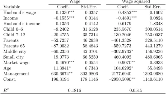
We employ the following instruments for the wage rate and its square. Speci…cally, we include the average market wage for women (Market wage), the age of the respondent (Age), and a dummy variable for being in a management position in a …rm (Management). To ensure su¢ cient variation in the average market wage for women, we specify the average market wage for women according to education, age, and the number of employees. The average market wage is expected to have a positive in‡uence on the wage rate of the respondent. Married women, however, tend to care not for the average market wage, but their own wage. Namely, the average market wage may have only indirect impacts on the individual’s time use through their own wage.
Age may proxy one’s business experience, accordingly it increases the wage. In the theoretical section of this paper, the location of the …rm explains di¤erences in wage rates. That is, …rms
located in the city centre o¤er higher wages than …rms located in the suburbs. However, this information is not reported in the JPSC. Instead, a dummy variable for Management is used as a proxy to control for this di¤erence. Pazy et al. (1996) noted that opportunities for senior position are not uniformly distributed in geographical space. Because management positions are senior positions, managers may only work in one location, typically the city centre. In empirical support, Daniels (1977) observed that all of the conurbation centres in the United Kingdom had lower levels of clerical employment in 1971 than in 1966. The evidence for administrators and managers, however, was more mixed, with the conurbation centres in Greater London, South- East Lancashire, and the West Midlands achieving a substantial increase in the numbers of these sorts of positions. Although this …nding is now rather dated, this study appears to suggest that married women in management positions are more likely to work in the city centre, meaning that they receive higher wages. Thus, wages and Management should be positively correlated.
To test the household responsibility hypothesis, past studies have speci…ed various house- hold characteristics as proxies for household responsibilities. Similarly to previous research, we include the number of children younger than 7 years (Child 0–6) and the number of children aged 7 to 12 years (Child 7–12) in Xi. In Japan, children aged 7 to 12 years attend primary school. If working mothers bear a greater share of child-care in the household, these variables decrease commute time with a corresponding increase in the time spent on housework. Lee and McDonald (2003) also included the presence in the household of parents or parents-in-law older than 59 years. They assumed that living with parents or parents-in-law may reduce the house- hold responsibilities of married women because of the assistance parents o¤er with child-care, housecleaning, meal preparation, etc. In fact, Lee and McDonald found that this particular variable decreases commute time. Ueda (2005) also included the presence in the household of the wife’s or husband’s mother aged 64 years or younger. However, this would estimate the housework time equation, not the commute time equation, as here. In the explanatory variables, Ueda (2005) also included the presence in the household of other parents, arguing that living with other parents may actually increase housework time, for example, by assisting the parents to eat or use the bathroom. In this analysis, we specify both the presence in the household of parents or parents-in-law aged 64 years or younger (Parents), and the presence in the household of parents or parents-in-law older than 64 years (Parents 65). We expect that Parents tends to be positively related to commute times, while it tends to be negatively related to housework times. Conversely, Parents 65 has a tendency to reduce commute times and increase housework
times.
Commute times also necessarily vary with the means of transport. For example, Nobis and Lenz (2005), Gould and Zhou (2011) and Olde Kalter et al. (2011) suggested that working women tend to use personal vehicles because their household support trips included shopping for groceries while the presence of accompanying children may lead them to favour the ‡exibility and convenience of an automobile. That is to say, a car is more likely to allow women to save on travel time. Srinivasan and Bhat (2005) found that wives in dual-income households with children with access to a personal vehicle spend more time on household chores than those who do not. They argued that this was because women without a personal vehicle may rely on public transportation or other means to commute; therefore, they are more likely to reduce the time spent on household chores. Unfortunately, the JPSC does not provide this kind of information.
Instead, three geographical categories are included, comprising 13 major cities in Japan (Large city), all other cities (Middle city), and towns and villages (Small city). In Japan, many people in large cities with a high population density commute by train or subway because the economies of scale entail lower commuting fares when using these transportation systems. In contrast, and because of lower population densities, car transport may be advantageous in middle- and small-sized cities. We expect that the estimated coe¢ cients for both Middle and Small will be negative in the commute times function and positive in the housework times function.
We should also con…rm whether the IV method modi…es the estimated coe¢ cients in our regressions. For that reason, we present the OLS estimates following the IV approach. We then estimate the time-use equations for husbands of Eq. (10), which have an identical structure to that of their wives because husbands simultaneously allocate their time use after considering the wife’s wage, the level of non-labour income, the number of children, etc. Third, we con-
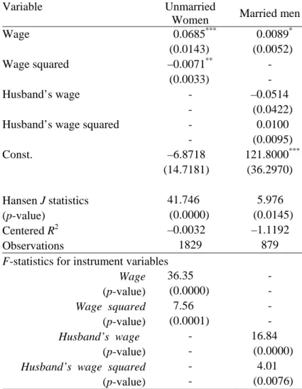
…rm whether the backward-bending hypothesis only applies to married women. To do this, we estimate the commute time equations using the observations for unmarried women and mar- ried men. Finally, we add a sample of married women working part-time to the …rst set of observations as a robustness check.
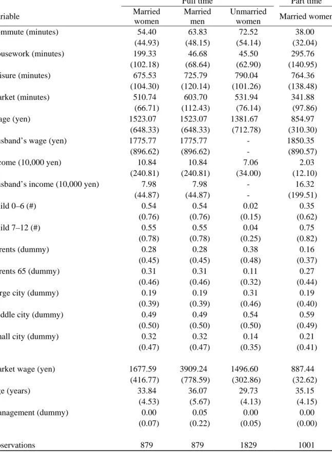
Table 1 provides summary statistics for the variables used in the regression analysis. The mean commute time of married women working full time is approximately 54 minutes, which is approximately 14 minutes longer than the average female commute time (including part- time workers) in the 1996 and 2001 STULA. Their mean housework time is approximately 199 minutes, which is approximately 3 minutes longer than the average female housework time.
The mean market work time is approximately 511 minutes, which is approximately 156 minutes longer than the average female market work time. Their mean wage rate is 1,523 yen. This is 153 yen lower than the mean market wage rate in the Basic Survey on Wage Structure (1993–2002) compiled by the Ministry of Health, Labour and Welfare.
The commute time of married men is approximately 9 minutes longer than that for women.
Married men spend only 47 minutes on housework per day, which is approximately 153 minutes shorter than that for married women. Our data thus suggest that wives have somewhat shorter commute times and much heavier household responsibilities. This is consistent with the litera- ture. Similar to married men, single women spend approximately 18 minutes longer on commute times and approximately 154 minutes fewer on housework times. The hours of housework for married women are then less likely to be ‡exible than either unmarried women or married men because of their relatively heavy household responsibilities. Therefore, adjusting commute time may become an important strategy for working married women to secure leisure time.9 Con- versely, it may be a somewhat less important issue for unmarried women and married men to reduce commute times. In fact, because of their relatively fewer domestic duties, these two groups spend much more time on leisure than do married women.
Table 1 also suggests that married women working part-time have the shortest commute and work times, whereas they have the longest housework time. The wages of part-time female workers are generally low. The data in Table 1 indicate that the average wage rate of part-time workers is roughly half that of full-time workers. Although we do not report this in the table, the standard deviation of the wage rate for part-time workers (310.30) is also smaller than that for full-time workers (648.33). Therefore, it may be inappropriate to test our hypothesis using only part-time workers. Our theoretical model, however, does not exclude part-time employment. If working time in the market is su¢ ciently small, and if both Eqs. (7) and (8) are negative, then a married woman is more likely to work and reside in the suburbs (Option 1), receive a low wage, and commute for only a short time. This appears to be also applicable for part-time workers.
Therefore, our hypothesis may still hold, even though we only add married women who work part-time to our sample.
9Kitamura (2010) collected 800 observations on full-time working dual-income households in the Tokyo Metropolitan area in Japan. Her survey results suggested that working mothers are more likely to reduce labour and commute times to secure homework time. This becomes more noticeable when the husband’s labour time is 10 hours a day or more.
4.2 Estimation results
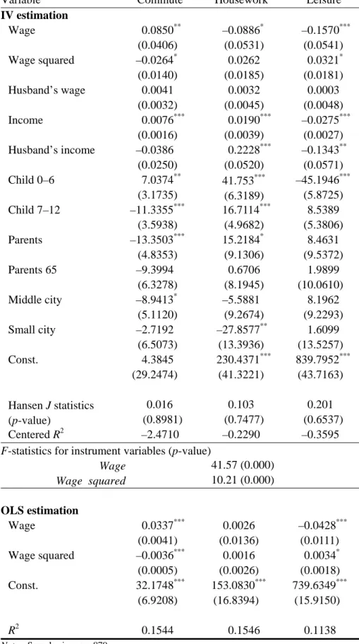
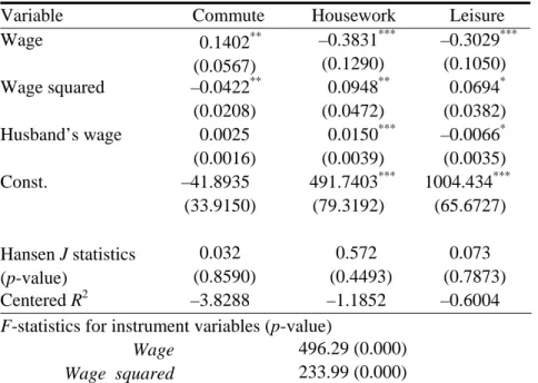
Table 2 provides the IV estimation results including F-statistics from the …rst stage that test the hypothesis that the instruments should be excluded from the …rst-stage regressions.10 All of the F-tests in Table 2 indicate that the instruments a¤ect Wage and Wage squared as all of theF-statistics are su¢ ciently large.
Before discussing the e¤ect of the wage rate on the time-use equations, we brie‡y refer to another control. Husbands appear to be unconcerned about their wife’s commute, housework, and leisure times, regardless of the wage level. The married women’s unearned income has a positive and signi…cant e¤ect on commute time. The unearned income of both wives and husbands has a signi…cantly positive impact on housework time and a signi…cantly negative impact on leisure time.
As expected, preschool-age children tend to increase housework time. Because child rearing takes time, married women must reduce leisure time. Preschool-age children, however, also increase the commute times of married women. This may be explained as follows. Households with small children choose to locate their home in the same suburb as their parents, because having one’s parents nearby may decrease the burden of child-care. Households then choose a suburb that o¤ers a better child-raising environment than the city centre. Alternatively, it might be di¢ cult to …nd a day care nursery in the city centre; therefore, households must choose to live in a suburb to obtain these services. Having a child aged between 7 and 12 years of age also has the expected e¤ect on the time allocation of married women. As the number of school-age children increases, greater household responsibilities result in shorter commute times and longer work times at home.
The estimated coe¢ cients for Parents display an unexpected sign in that while households with parents or parents-in-law aged 64 years or younger may decrease commute times, they also increase housework time. These results are inconsistent with Lee and McDonald (2003). One possible interpretation is that (altruistic) children tend to live with their parents when parents have a problem with deteriorating health. Consequently, children must increase the time they make available for nursing care (Johar et al. 2010). Alternatively, perhaps (sel‡ess) children spend large amounts of time performing nursing care to acquire a parent’s dwelling in the future (Yamada 2006). The coe¢ cients of Parent 65 have the expected sign, but are statistically
1 0The estimation results for the …rst stage, namely, wage rates and its square, are given in electronic supple- mentary material. All instruments indeed exert a signi…cantly positive impact on wage rates.
insigni…cant.
Married women in middle-sized cities that commute by vehicle rather than by rail appear to have shorter travel time to work. The small-city dummy also displays a negative sign, although it is insigni…cant. In contrast to Srinivasan and Bhat (2005), proxy dummies for automobile commuters (middle- and small-city dummies) are negatively related to housework time, but are only signi…cant for small cities. Finally, the constant term in column 2 (Housework) suggests that the married women in our sample appear to spend long hours on domestic chores (about four hours of housework).
The wage rate of married women and its square on the time spent commuting are important for our main argument. As expected, the wage rate has a signi…cant and positive impact on commute time while the square of the wage rate has a signi…cant and negative impact on commute time. Therefore, the estimation result appears to indicate a non-linear relationship between the wage rate and commute time. Wage has a signi…cant and negative impact on housework time. That is, an increase in the wage rate reduces any additional housework time because it tends to be more attractive for the married woman to work in the market than at home to obtain consumer goods. We can con…rm that some simple and routine home-produced goods and services, such as cooking, cleaning, washing, and shopping, are substitutes for market- purchased goods. Wage squared is positive, but insigni…cant. The insigni…cant impact of Wage squared implies that highly paid wives leave most of their housework responsibilities to the market. The implication is quite natural in family economics model, especially when home goods and market goods are perfect substitutes, as discussed in Section 3 (Bryant and Zick 2006). However, this result contradicts Prashker et al. (2008), who suggested that women with higher income levels are more likely to reduce commute times to retain housework time.
Column 3 (Leisure) indicates that leisure time follows a C-shaped pattern in accordance with wage increases.11
We should also con…rm whether the IV method modi…es the estimated coe¢ cients. Table 2 provides the OLS estimation results using the same observations. However, only the estimates for the female wage rate variables and the constant term are reported. Comparing the two results demonstrates that the absolute estimated values of wage and wage squared in the IV
1 1We divide leisure time into the original categories and estimate these time equations. The estimation results indicate that the increase in wage rates decreases the time spent on hobbies, recreation, social life (v), and personal care (vi), and increases the time spent on study (iii). All of the coe¢ cients for Wage squared are statistically insigni…cant.
estimation are larger than in the OLS estimation. This suggests that OLS under-estimates the e¤ect of the wage rate on the time-use allocation compared with the IV method.
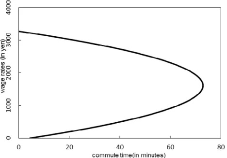
Using the estimated coe¢ cients of Wage, Wage squared, and the constant term in columns 1 (Commute) and 3 (Leisure) of Table 2, Fig. 2 (a) depicts the relationship between commute time and wage rates for married women, while Fig. 2 (b) shows the relationship between leisure time and wage rates. Fig. 2 (a) indicates that the e¤ect of wage rates on commute time indeed follows a backward-bending pattern. Therefore, married women with either a low or high wage rate may locate their residence closer to the location of their employment. In contrast, married women with wage rates between these extremes tend to choose longer commutes because they may not have su¢ cient wages to move to the new location. Using this …gure, we can see that commute time peaks at approximately 1,610.72 yen, which is 87.65 yen higher than the average wage rate in Table 1.12 Fig. 2 (b) shows that married women with high wage rates attempt to secure leisure time by decreasing their commute time. In contrast, married women with middle-level wages are obliged to reduce leisure time because of long commutes with household responsibilities. Using data on Italian females, Meloni et al. (2009) concluded that women who have longer commutes devote less time to recreation and leisure. Our empirical results suggest that the negative relationship between leisure and commute times tends to be through wages.
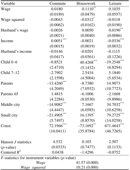
Table 3 provides the IV estimation results for husbands working full time. As shown, the wage rates of wives have no signi…cant e¤ect on the commute and leisure times of their husbands.
The housework time of husbands, however, follows an inverse C-shaped pattern. In other words, husbands perform slightly more housework when wives earn middle-level wages, which may re‡ect the fact that these wives have the longest commute times in our sample.
4.3 Comparison
The empirical section appears to indicate that the commute time of married women follows a backward-bending pattern, as hypothesized by the theoretical model. This section investigates whether this hypothesis also applies to unmarried women and married men. We do not consider unmarried men as they are not included in the JPSC.
Our theoretical model can easily apply to unmarried women as we assume an additive form of the utility function. The only di¤erence then between married and single women is the presence
1 2The result using OLS shows that commute time peaks at approximately 4,733.91 yen, notwithstanding that 99.54% of married women earn less than this. Therefore, commute time tends to become an increasing function within a reasonable range.
of the husband’s wage rate in Eq. (8). That is,wM does not exist for single (unmarried) women.
This implies that an unmarried woman is less likely to choose Option 3 than a woman in a married couple because she does not consider the man’s opportunity cost of long commuting. Thus, the commute time of unmarried women may bend backwards more slowly than the commute time of married women. Furthermore, although the theoretical model focuses on married women, let us replace all parts for married women with married men, and vice versa. We could then hypothesize that the commute time of married men may also follow a backward-bending pattern.
To test these hypotheses, we estimate the time-use equations model for both single women and married men working full time. These are similar to the married women’s model. However, only the wage rate variables and the constant term are reported in Table 4. Similar to married women, the commute time of single women follows a backward-bending pattern. Comparing Tables 2 and 4, we …nd that the absolute value of the coe¢ cients of Wage squared for unmarried women is substantially smaller than that for married women, while the coe¢ cients for Wage have relatively similar values. This suggests as expected that the commute time of unmarried women tends to bend backwards more slowly than the commute time of married women. However, the commute time of unmarried women is almost increasing with respect to wage rates within a reasonable range, because commute time peaks at approximately 4,823.94 yen, even though 98.85% of unmarried women earn less than this value. As a result, the commute time does not appear to bend backwards. In contrast, both the husbands’ wage rates and its square in column 2 (Married men) have no impact on commute time. Husbands appear to spend long hours commuting because the signi…cantly positive constant term suggests approximately two hours, regardless of the wage level, within any normal level.
In sum, the empirical results appear to suggest that the commute time of both unmar- ried women and married men do not follow a backward-bending pattern, presumably because household responsibilities are not signi…cant for either married men or unmarried women.
4.4 Robustness check
To this point, we have ignored married women working part-time. In this section, we include married women working part-time to our sample in Table 2. Table 5 provides the IV estimation results for married women in both full- and part-time work. As expected, the e¤ect of the wage rate on the commute time of married women again follows a backward-bending pattern. Our hypothesis is then robust, even though married women employed part-time are included in our
sample. Because part-time workers are included, the constant term for housework time in Table 5 becomes substantially larger than in Table 2. Similar to column 2 (Housework) in Table 2, column 2 (Housework) in Table 5 suggests that wives reduce housework time in accordance with wage increases; that is, Wage has negative and signi…cant coe¢ cients. Interestingly, further increases in wage rates increase housework time because Wage squared is signi…cantly positive.
This is quite di¤erent from Table 2. The C-shaped pattern of housework time implies that both married women with high wages and married women with low wages devote more time to household responsibilities. Consistent with Prashker et al. (2008), working wives with high wages retain housework time by reducing commute times. Another possible interpretation is that full-time working mothers with high wages appear to feel guilt over their inability to ful…l specialized housework roles, such as child-care (Hofmeister 2005; Kim and Ling 2001; Lee 2002);
thus, they attempt to spend more time on child rearing as wage rates rise.
5 Discussion
There are several ancillary items of note in the current analysis. First, it is quite odd that the wage rates of married men play no role in the commute time equations. Although a few studies have clari…ed that the location decisions of dual-income households are more sensitive to the wife’s earnings than that of the husband’s, the latter has at least some impact. However, married men’s wages may have an in‡uence on commute time if we employ alternative models, such as a bargaining or search model. In a bargaining model, the relative wages of wives coupled with that of their husbands play an important role in determining the time use of couples (Friedberg and Webb 2005). To consider this, we tentatively attempt to explain the commuting time of wives in terms of the relative wages of wives coupled with that of their husbands and the squared wage.
At the estimation stage, we exclude the wage rate of wives and their squared wage, and the wage rate of their husbands. The OLS estimation results indicate that the estimated coe¢ cient for the relative wage is positive while that for its squared value is negative. Using the coe¢ cients, we …nd that the commute times of married women tend to bend backwards when the relative wage reaches approximately 2.90. Alternatively, in a search model, the spatial moving behaviour of dual-income households depends on the distance between their workplaces (van Ommeren et al. 1998).
Second, we have access to panel data but pool it over time to provide a single cross-section of data because of the otherwise limited sample size. Because changing the place of residence