3次元多様体から平面への安定写像の1次半局所不変 量

九州大学学術情報リポジトリ

Kyushu University Institutional Repository

3次元多様体から平面への安定写像の1次半局所不変 量

山本, 稔

http://hdl.handle.net/2324/454845

出版情報：Kyushu University, 2003, 博士（数理学）, 課程博士 バージョン：

権利関係：

l

..

FIRST ORDER SEMI-LOCAL INVARIANTS OF STABLE MAPS OF 3-MANIFOLDS INTO THE PLANE

MINORU YAMAMOTO

ABSTRACT. In the late 1980's, Vassiliev introduced new graded numerical invariants of knots, which are now called Vassiliev invariants or finite~type invariants. Since his definition, many people have been trying to construct Vassiliev type invariants for various mapping, spaces. In the early 1990's, Arnold and Goryunov introduced the notion of first order (local) invariants of stable maps.

In this paper, we define and study first order semi-lor;:al invariants of stable maps and those of stable fold maps of a closed orientable 3-dimensional manifold into the plane.

Here, a stable fold map is a stable map with only fold singular points and a first order semi-local invariant is an isotopy invariant which is constructed by looking at the singular value set locally and the singular fibers semi-locally. We show that there are essentially seven first order semi-local invariants. For a stable map, six of them count the number of singular fibers of a given type which appear discretely (there are exactly six types of such singular fibers), and the other one is the rotation number of the singular value set.

Besides these invariants, for stable fold maps, the Bennequin invariant of the singular value set corresponding to definite fold points is also a first order semi-local invariant.

Our study of codimension 1 unstable fold maps provides invariants for the connected components of the set of all fold maps.

1. Introduction 1.1. History 1.2. Purpose

1.3. Organization of the paper 1.4. Acknowledgment

2. Classification of mulh-germs 2.1. A-equivalence of multi-germs 2.2. Classification of multi-germs

CONTENTS

3. Stable maps and unstable maps of codimensions one and two 3.1. Stable maps

3.2. Unstable maps of codimensions one and two

2000 Mathematics Subject Classification. Primary 57R45; Secondary 32S20, 58Kl5.

The author has been supported by JSPS Research Fellowships for Young Scientists.

1

2 2 3 4 6 6 6 7 9 9 11

2 MINORU YAMAMOTO

3.3. Bifurcation diagrams 14

4. Classification of singular fibers 17

4.1. Definition of an equivalence of fibers 17

4.2. Classification of singular fibers of stable maps 19

4.3. Classification of unstable maps of ·codim_ensions one and two 22

4.4. Coorientations of codimensiori one strata 24

5. The Vassiliev cochain complex for the weak equivalence 25

6. First order semi-local invariants 27

6.1. Semi-local invariants 27

6.2. First order semi-local invariants 28

7. First order semi-local invariants of stable maps 30

7.1. Computation of the coboundary operator 30

7.2. Geometric interpretations of the 1-cocycles 31

7.3. Surgical rotation number 32

7.4. Proof of Theorem 7.3(7) 33

7.5. Linear independence of the first order semi-local invariants 33 8. A non-local first order invariant of stable maps 36 9. First order semi-local invariants of stable fold maps 40 9.1. Computation of the Vassiliev quotient cochain complex for fold maps 40 9.2. Geometric interpretations of the 1-cocycles in Ker( JF) . 42

9.3. Bennequin invariant 43

9.4. Proof pf Theorem 9.4 (7) 44

10. Invariants of the connected components of the space of fold maps 47

References 50

1. INTRODUCTION

1.1. History. Vassiliev [50] introduced a wonderful method to define graded numerical invariants of knots, which are now called Vassiliev invariants or finite-type invariants. He constructed these invariants by carefully studying a certain stratification of the mapping space C⁰⁰(S¹) R^3). Since his definition, many people ha~e been trying to construct Vas- siliev type invariants for various mapping spaces. Arnold [4] introduced "basic invariants"

(we call them Arnold invariants) for stable immersions of S¹ into R^2, which brought a new insight to the classical subject of the topology/geometry of plane curves. Arnold invariants are regarded as a special kind of first order Vassiliev type invariants, which are objects of great interest by themselves. Arnold invariants of plane curves (and those of wavefronts) were studied by many authors, for example, Aicardi [2], Goryunov [17L ·

FIRST ORDER SEMI-LOCAL INVARIANTS OF STABLE MAPS 3

Tchernov [46, 47], etc. The construction of this kind of order one invariants may work for stable maps of manifolds whose dimensions are greater than 1. In fact, as a kind of a generalization of the ]±-invariants (not involving the strangeness invariant

St),

Goryunov

[16]

introduced and studied first order local invariants of stable maps of an oriented closed surface into R^3. Aicardi and Ohmoto [3] worked on first order local invariants of stable maps of a closed surface into R² (see also [391). It should be remar~ed that in both cases) these first order "locaP' invariants are determined by numerical invariants of discrete criti- cal sets and a certain Bennequin invariant of the critical value set (note that this is related to the J+-theory of plane curves). See Remark 6.5 for the other results about Vassiliev (finite) type invariants. In these works, almost all invariants are essentially reduced to order one invariants.

1.2. Purpose. In this paper, we consider the case where the source manifolds are closed orientable 3-dimensional manifolds and the target manifold is the plane. In all the cases mentioned in the previous subsection, the dimensions of the target manifolds are greater than or equal to those of the source manifolds. Thus for any point in the target manifold₁ the inverse image of this point consists of a finite number of points, provided that the map is proper and generic enough. Hence, in order to study first order (local) invariants of such stable maps, we have only to consider multi-germs along zero dimensional sets. However, if the dimension of the source manifold is strictly greater than that of the target manifold, then the inverse image of a point (or the fiber over a point) is no longer a discrete set.

In general, this forms a complex of.positive dimension. Hence, if we consider multi-germs orily along singular points in a fiber to study first order invariants of stable maps, then it is expected that little information about stable maps appears in these invariants. Thus, to get much information about stable maps from first order invariants, we need to .study map germs along a whole fiber of positive dimension.

We define and study first order semi:.local invariants of such stable maps. A first order semi-local invariant is a special kind of a first order invariant: when a homotopy in the mapping space crosses a codimension 1 stratum transversely at a codimension 1 unstable map, the jump of the invari:ant is determined by the homeomorphism type of the local deformation of the singular value set near the .codimension 1 singular value and by the diffeomorphism types of associated singular fibers. Note that the notion of a diffeomorphism of singular fibers modulo regular components was first used implicitly by Kushner, Levine and Porto [26,

29].

After that Saeki

[45]

gave a precise definition of this notion (including regular components).

This is the first study of first order invariants when the dimension of the source manifold is strictly greater than that of the target manifold) as long as the author knows.

..

4 MINORU YAMAMOTO

1.3. Organization of the paper. The paper is organized as follows.

In Section 2> we review the classification of multi-germs (R ^3, S) -+ (R ^2, y) up to A- equivalence (i.e., C⁰⁰ right-left equivalence)) where S is a set of finitely many isolated points. We list the A-equivalence classes of miniversal unfoldings of such multi-germs whose parameter spaces have dimensions 0, 1 or 2. They were studied by Rieger-Ruas [41], Gibson-Hobbs [14], Nabarro [35] and Rieger [40], and we use their results in this paper.

We have to add two exceptional A-equivalence classes of miniversal unfoldings of multi- germs which correspond to

D;

or a quadruplefold. The reason is as follows. Miniversal unfoldings of these multi-germs have parameter spaces of dimension 3. However, their A-modalities are all equal to 1. On the parameter space R³ of their miniversal unfoldings, one coordinate t of the coordinates (a, b, t) E R³ corresponds to the A-modality. Thus Dt

and a quadruplefold ai:e considered to be 1-parameter families of A-equivalence classes.

To obtain first order invariants, we have to consider each such 1-parameter family to constitute a stratum, and the codimension of each such stratum is equal to 2. For details, see [40] and Subsection 2.2.

In Section 3, we define stable maps and unstable maps of codimensions 1 and 2. By using the classification of miniversal unfoldings of Section 2, we study local deformations of singular value sets and the associated local singular fibers near singular points.

In Section 4, we first define the notion of the weak equivalence for singular fibers (preim- ages of singular values). This equivalence relation reflects homeomorphis·m types of (local deformations of) singular value sets and diffeomorphism types of the associated semi-local singular fibers. This equivalence relation is related to the C⁰⁰ equivalence for map germs · along singular fibers. See [45] for the definition of the 0⁰⁰ equivalence. Since our equiv- alence is weaker than the C⁰⁰ equivalence, we use the term "weak" for our equivalence relation. We classify singular fibers of stable maps and unstable maps of codimensions 1 and 2 up to this equivalence relation (see Theorems 4.4, 4.7 and 4.8). For a stable map, there are exactly six weak equivalence classes of singular fibers which appear discretely.

Then, we define the equivalence relation, which we also call weak equivalence for simplic- ity, for unstable maps of codimensions 1 and 2 and classify them up to this equivalence.·

relation. We then define the coorientation of each weak equivalence class of codimension 1 unstable maps by looking at the local deformation of its singular value set and the associated (semi-local) singular fibers.

In Section 5, we construct the Vassiliev cochain complex for the weak equivalence classes of unstable maps of codimensions 1 and 2. (As general references about the Vassiliev co chain complex, see [23, 49].)

..

FIRST ORDER SEMI-LOCAL INVARIANTS OF STABLE MAPS 5

In Section 6, we define.first order semi-local invariants of stable maps. These invariants are constructed from the cocycles of the Vassiliev cochain complex mentioned above and they are isotopy invariants of stable maps.

In Section 7, we determine the first order semi-local invariants of stable maps by using the Vassiliev cochain complex constructed in Section 5 (see Theorem 7.2). More precisely, we show that there are essentially seven first order semi-local invariants of stable maps.

By a careful study of homotopies which intersect co dimension 1 strata ( the hypersurface in the mapping space which consists of the co dimension 1 unstable maps) transversely, we give geometric interpretations of all the invariants. It turns out that for a stable map, six of them count the number of singular fibers of a given weak equivalence class which appear discretely (there are exactly six such weak equivalence classes by Theorem 4.4) and the other one is the "rotation number" of the singular value set (see Theorem 7.3).

Then we construct several explicit examples of stable maps

f :

S³ --t R^2• By using these examples, we show that the above seven first order semi-local invariants together with a (non-zero) constant invariant are linearly independent for stable· maps of an arbitrary closed orientable 3-dimensional manifold.

Note that these types of results would be impossible if we used the multi-germ of a given map only along the singular points in a fiber instead of considering the map germ along a whole singular fiber.·

In Section 8, we subdivide the weak equivalence classes of unstable maps of codimen- sions 1 and 2 by using a global property of such maps. To subdivide them, we look at their singular value sets globally. By using such a finer classification> we give an additional first order invariant of stable maps₁ which is a non-local invariant, and give a geometric interpretation of this invariant (see Propositions 8.1 and 8.2).

In Section 9, we consider the space of all fold maps. A fold map is a smooth map with only fold singular points. By using the Vassiliev cochain complex for the weak equivalence classes of unstable fold maps of codimensions 1 and 2, we determine the first order semi- local invariants of stable fold maps and give geometric interpretations of all the invariants (see Theorems 9.3 and 9.4).

By combining our results with other results about first order invariants which are al- ready known, we may conjecture that first order invariants can give information only about the 0-dimensional strata of the critical value set, endowed with the topology of the associated fibers, or the topology of the critical value set ( e.g. the rotation number or the Bennequin invariant).

In Section 10, we give several invariants for the connected components of the space of all fold maps. These invariants are obtained by a careful study of codimension 1 unstable fold maps carried out in the previous sections.

..

6 MINORU YAMAMOTO

Throughout the paper, all manifolds and maps are differentiable of class C^00•

1.4. Acknowledgment. The author would like to express his sincere gratitude to Prof.

Osamu Saeki, Prof. Toru Ohmoto, Prof. Joachim Rieger and Prof. Maria Ruas for their invaluable comments and encouragement.

2. CLASSIFICATION OF MULTI-GERMS .

In this section, we quickly review the classification of multi-germs by A-equivalence ( that is, C⁰⁰ right-left equivalence).

2.1. A-equivalence of multi-germs. In this subsection, we review some fundamental concepts and results from singularity theory. For details, see [5, 10, 39, 51].

Let

f :

(M, S) ----+ (R², y) be a multi-germ at finitely many isolated points S of

J-

¹(y), where M is a 3-dimensional manifold. When S consists exactly of one point, we also say that

f

is a mono-germ. An unfolding of such a multi-germ

f : (

M, S) ----+ (R², y) with parameter space Rs centered at t0 E Rs means a multi-germ F: (M x R5, S x {t₀})---+

(R², y) such that F(x, to)=

f

(x).

Let Mi be 3-dimensional manifolds (i

=

1, 2). Let

Ji :

(Mi, Si) ---+ -(R2, Yi) be multi- germs and Fi : (Mi x Rs, Si x {ti}) ^----+ (R², Yi) unfoldings of fi with parameter space R.⁸ centered at ti ( i

=

1, 2). We say that F1 and F2 are A-equivalent if there exist a diffeomorphism germ ip: (R8,t1)---+ (RS,t2), and unfoldings

R:

^(M1 x R8,S₁ x {t1})---+

(M2 , S_{2 )} and

L :

^{(R2 x RS, (y}1 , t1)) ---+ (R², y_{2 )} of diffeomorphism germs R: (M_{1 ,} S₁₎ ---+

(M2, S2) and L : (R², Y1) ---+ (R\ y2 ) respectively, such that the following diagram is commutative:

(M1 X RS, S1 X { t1}) ^{- - + F1} (R2 x Rs, (Y1,t1)) ^{--'----+ 1r} (RS,

t

_{1 )}

(R,'P)

1

^(L,,p)

1 _'Pl

(M2 X R5,S2 X {t2}) ^{- - + F1} (R² x Rs, (Y2,t2)) ^{- - + 1r} (R8,t2).

Here, 1r is the projection to the secon~ factor, (

R,

^{'P) ( or}

(L,

cp)) is defined by (

R,

'P) (x, t) ~ (R(x, t), rp(t)) (resp. by (L,

i.p)(y,

t)

=

(L(y,

t),

cp(t))), and the map Fi, i

=

1, 2, is defined

- ^.

by Fi(x, t)

=

(F;(x, t); t).

Two unfoldings

Fi

and F2 of

f : (

M, S) ---+ (R ², y) with the same parameter space Rs are said to be !-isomorphic if Fr and F₂ are A-equivalent with Rand L being the identity multi-germs idM and idR2 respectively.

Let F: (M x Rsi,s x {t_{1 }) -} (R²

,y)

be an unfolding off: (M,S) ^----+ (R²

,y)

and g : (R^52, t_{9 )} ---+ (R^81,

t

f) a smooth map germ. We define the induced unfolding g* F: (M X R⁵2, S x { t_{9 })} ---+ (R2, y) by g* F(x,

w) =

^F(x, g(w)), which is also an unfolding

..

FIRST ORDER SEMI-LOCAL INVARIANTS OF STABLE MAPS 7

of

f.

An unfolding F of

f

is called a universal unfolding if any unfolding G of

f

is

!-

isomorphic to an unfolding induced from F. A universal unfolding of a multi-germ

f

is called a miniversal unfolding if the parameter space has the minimal dimension among all universal unfoldings of

f.

For a multi-germ f: (M) S)--+ (R², y)> let B(f)s denote the set of

c=

vector fields along

f.

That is, it is the set of multi-gerrr.is ( : (M, S) --+ TR² such that ((x) E TRJ(x) (x E M).

We set (}(M)s

=

B(idM ^)s and (}(R²)y

=

B(idR2 )y·· The two maps tf: ~(M)s--+ B(f)s and wf : B(R²)y --+ B(f)s are defined by tf(,;)

=

dj o,; and wf(r,)

=

r, of respectively. The

extended tangent space T

Aef

is defined by

T

Ae! =

tf (e(M)s)

+

w

f

(B(R²)y)

c

B(f)s

and the dimension of the quotient vector space 8(!)3/T Aef is called the Ae-codimension off.

Note that. if the Ae-codimension of

f

is finite, then it admits a universal unfolding and the Ae-codimension coincides with the dimension of the parameter space of a miniversal unfolding off (see [39, 51]). A multi-germ

f :

(M, S) --+ (R², y) is said to be Ae-finite if the Ae-codimension of

f

is finite. It should be noted that every Ae-finite multi-germ is finitely determined. That is, its A-equivalence class is determined by its ~et of finite order, and hence it is represented by a polynomial multi-germ (see [51]).

2.2. Classification of multi-germs. Let us consider the classification of those A-finite multi-germs whose Ae-codimension minus A-modality is strictly less than three. In the following, let·mA(f) E Z denote the value of (Ae-codimension)-(A-modality) for

f.

^The

modality is defined as follows. Suppose that a Lie group G acts on a variety V, then a theorem of Rosenlicht [42] implies that V has a uniquely determined finite stratification S such that the action of G on each stratum S defines a fibration S --+ S/G. If a point p E V is in a stratum S such that dim S/ G

=

m, then we say that the modality of p E V is equal to m E Z2:o, where Z2:o is the set -of non-negative integers. The A-modality of an Ae-finite mono-germ/:

(R

^3, x)--+

(R2,

y) is the modality of an A-sufficient jet jk fin Jk(3, 2)x,y under the action of the Lie group Ak of k-jets of elements of A. If

f

is not a mono-germ, then we can define the A-modality similarly. For details, see [40, 52].

Let f :

(R

³, S) --+

(R2,

0) be an Ae-finite multi-germ, where S ~s a set of finitely many isolated points of

J-

¹(0). To determine first order invariants of stable maps, we may assume that ^mA (f) is equal to 0, 1 or 2.

For

f

with mA (!)

=

0, 1 or 2, the A-equivalence classification of mono-germs an1 their miniversal unfoldings has been obtained by Nabarro [35], Rieger [40], and Rieger-Ruas [41]. The A-equivalence classification of multi-germs and their miniversal unfoldings has- been studied by Gibson-Hobbs [14]. In fact, they considered multi-germs

f :

(R², S) --+

(R²) 0) and classified them by A-equivalence. We can use similar arguments for multi- germs

f :

(R³, S) --..:., (R²) 0) and obtain the required A-equivalence classification.

Let

f :

(R3, S) - (R2, 0) be a multi-germ .. We put S(f)

=

{q E R³

I

rank dfq < 2}

and call it the singular set germ of f. Furthermore, we call

f

(S(J)) the singular value

·set germ off,

Let

f : (R3,

S) --+

(R

^2; 0) be a multi-germ such that S C S(f) and mA(f) :::; 2. Then we have S

= {

^q1 , . . . , qk}, 1 :::; k :::; 4, and there exist local coordinates (xi) Yi, zi) and (X, Y) around qi E R³, 1 :::;

i:::;

k, and

f

(qi)

=

0 E R² respectively such that a miniversal unfolding of

f

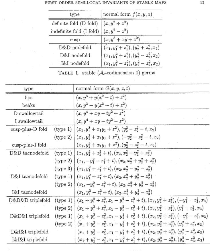
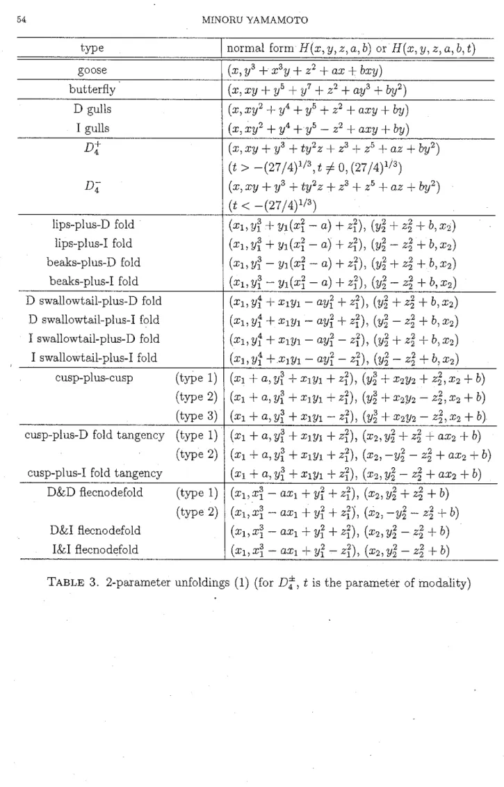
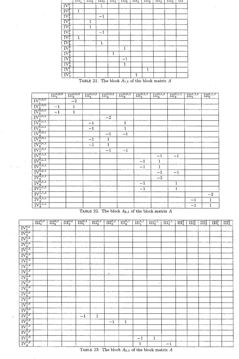
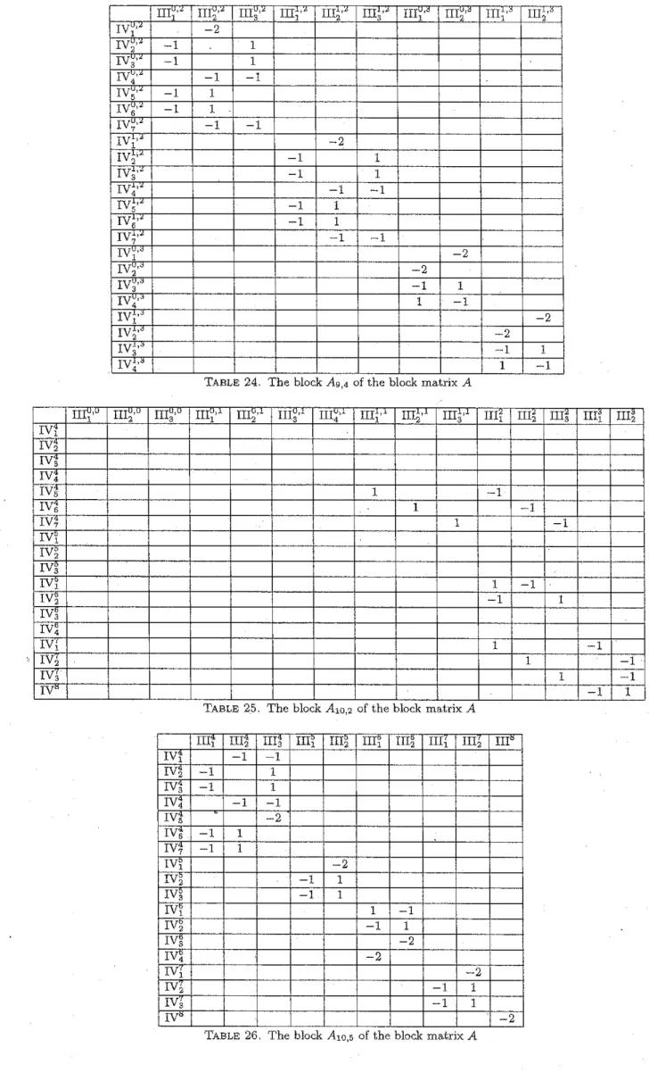
is expressed by one of the polynomials listed in Tables 1-5 with respect to the local coordinates.

I

Table

111

Table 2

I I

Table 3

I

ITable 4

I I

Table 5 !

We remark that by [14, 35, 40, 41], Tables 1-5 give the complete list of A-equivalence classes of multi-germs

f :

(R³, S) --+ (R2, 0) such that SC S(f) and mA(f) :::; 2. In our situation, the Ae-codimensions of

D;

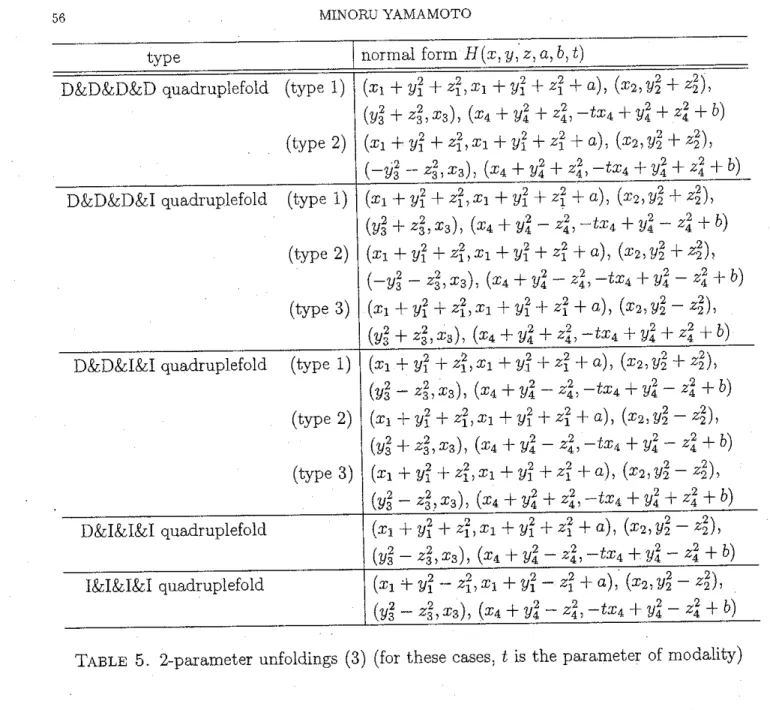
and a quadruJ)lefold are equal to 3 and their A-

modalities are equal to 1. For the miniversal unfoldings for these cases t is the parameter

· of modality in Tables 3 and 5. For the other classes, their A-modalities are equal to 0.

Let

f :

(R^3, S) -> (R^2, 0) be a stable germ in Table 1. Then using the local normal forms in Table 1, we see that the singular value set germ f(S(f)) around O is as depicted in Figure 1, where (1) corresponds to a fold point, (2) corresponds to a cusp point, and (3) corresponds to a nodefold.

I

Figure

11

Let G : (R³ x R, S x {O}) -> (R², 0) be a I-parameter unfolding in Table 2. We define 9t: R^{3 ---+} R² by 9t(q)

=

G(q)t). Suppose that OE g₀(S(g_{0 ))} and SC S(g_{0 ).} Then using the local normal forms in Table 2, we see that the deformations of the singular value set germ 9t(S(gt)) around O are as depicted in Figure 2> where (1) corresponds to lips, (2) corresponds to beaks, (3) corresponds to a swallowtail) ( 4) corresponds to a cusp-plus-fold, (5) corresponds to a tacnodefold and (6) corresponds to a triplefold.

I

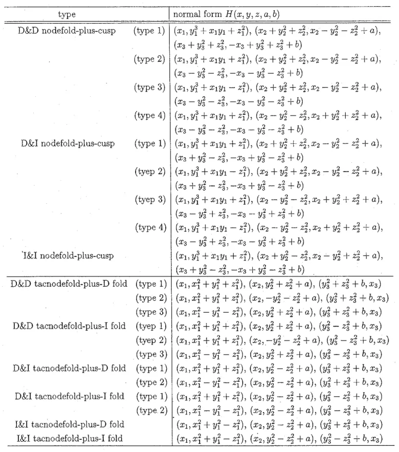
^{Figure 2 j}

Let H ·: (R³ x R², S x {(O, O)}) ---+ (R², 0) be a 2-parameter unfolding in Tables 3 or 4 other than Df. We define ha,b : R³ -> R² by ha,b(q)

=

H(q) a, b). Suppose that O E ho,o(S(ho,o)) and_S C S(ho,0 ). Then using the local normal forms in Tables 3 or 4, we see that the deformations of the singular value set germ ha,b(S(ha,b)) around O are as depicted ih Figure 3. Let H: (R^{3 X} R³,S X {(0,0)0)})--+ (R²,0) be a 3-parameter unfolding in Tables 3 or 5 which corresp·onds to

Dt

or a quadruplefold. We fix

t =

Jo E R in the corresponding local normal form and define ha,b : R³ ---+ R² by ha,b(q) - H(q, a, b, t0 ).

Suppose that O E h0,0(S(ho,o)) and S C S(h0,0 ). Then using the local normal forms,

,.

FIRST ORDER SEMI-LOCAL INVARIANTS OF STABLE MAPS 9

we see that the deformations of the singular value set germ ha,b(S(ha,b)) around O are as depicted in Figure 3. In Figure 3, (1) corresponds to a goose, (2) corresponds to a butterfly, (3) corresponds to gulls, ( 4) corresponds to

Dt,

⁽⁵⁾ corresponds to D

4,

⁽⁶⁾

corresponds to a lips-plus-fold, (7) corresponds to a beaks-plus-fold, (8) corresponds to a swallowtail-plus-fold, (9) corresponds to a cusp-plus-cusp, (10) corresponds to a cusp-plus- fold tangency, (11) corresponds to a flecnodefold, (12) corresponds t<;, a nodefold-plus-cusp,

(13) corresponds to a tacnodefold-plus-fold, and (14) corresponds to a quadruplefold.

I

Figure ³

I

In Figure 3, on each 2-dimensional region R of the parameter space, we have depicted ha,b(S(ha,b)) C R² for (a, b) E R. Some parameter spaces in Figure 3 may not strictly coincide with the corresponding (a, b)-plane for Hin Tables 3-5. For each of these cases, we need to compose an orientation preserving homeomorphism on the (a, b)-plane to obtain the corresponding parameter space in Figure 3.

3. STABLE MAPS AND UNSTABLE MAPS OF CODIMENSIONS ONE AND TWO

In this section, we define stable maps and unstable maps of codimensions 1 and 2 by using the A:..equivalence classification of multi-germs as in Tables 1-5. We also study local behaviors of their singular value sets and their singular fibers.

Let

f :

M --+ R² be a smooth map. We set S(f)

=

{q E M

I

rank dfq < .2} and call it the singular set off. Furthermore, we call f(S(f)) the singular value set off.

When y E R² is in the singular value set off : M--+ R², we call

J-

^1(y) a singular fiber;

otherwise, a regular fiber.

3.1. Stable maps. Let M be a closed 3-dimensional manifold and

f :

M ---+ R ² a smooth map. We denote the set of such maps by C⁰⁰(M, R²) which is equipped with the Whitney C⁰⁰-topology. A smooth map

f

is said to_be stable if in C⁰⁰(M, R^2), there exists an open neighborhood U of

f

such that for any g E U, g is C⁰⁰ right-left equivalent to

f,

that is, there exist two diffeomorphisms <l> : M --+ M and cp : R² ---+ R² such that the following diagram is commutative:

-

'P

It is known that the set of stable maps is open and dense in C⁰⁰(M, R²⁾ (see [32]). Note that fo.r a stable map

f :

M ^--+ R^2, S(f) is a compact 1-dimensional submanifold of M. The following characterization of stable maps is well-known (see [15, 26, 29, 53] and Table 1).

Proposition 3.1. A smooth map

f :

M ---+ R² of a closed 3-dimensional manifold into the plane is stable if and only if the following conditions are satisfied.

(i) For every q E M₁ there exist local coordinates (x, y, z) and (X, Y) around q E M and

f

(q) E R² respectively such that one of the following holds:

(X of, Yo f)

=

(x) y), (x, y2

+

zz), (x, y2 - zz),

q :regular point, q :definite fold point, q:indefinite fold point, (x, y³

+

xy

+

^z2), q:cusp point.

(ii) For every y E f(S{1))₇

J-

¹(y) nS(f) consists of at most two points and the multi- germ (f!S(f),

1-

¹(y) n S(f)) is right-left equivalent to one of the three multi- germs as depicted in. Figure 1: (1) represents a single immersion germ which corresponds to a fold point₁ (2) corresponds to a cusp point1 and (3) represents a normal crossing of two immersion germs each of which corresponds to a fold point.

Suppose that for a stable map

f :

M -> R ², there are distinct singular points q₁ and q2 in S(f). such that y

= f

(q1)

=

f (q2) ^E R² ·holds. In this case, we call y a nodefold off or a node off (S(f)). Note that S(f) is a closed 1-dimensional submanifold of M> that the number of nodefolds of

f

is finite and that the number of cusps on each component of S(f) is even (see [27]).

Definition 3.2 ([45)). Let Mi be manifolds and Ai C Mi subsets, i

=

0, 1. A continuous map g : Ao ---+ A₁ is said to be smooth if for every point q E A_{0 ,} there exists a smooth map

g:

V---+ M₁ defined on a neighborhood V of q in Mo such that

glV

nAo

=

g\V

n

Ao. Furthermore, a smooth map g : Ao ---+ A₁ is a diffeomorphism if it is a homeomorphism and its inverse is also smooth.

Let q be a singular point of a stable map

f :

M ---+ R^2. Then) using the local normal forms in Table 1, we. can easily describe the diffeomorphism type of a neighborhood of q in

J-

¹(f (q)). That is, we easily get the following local characterization of singular fibers.

Lemma 3.3. Let

f :

^{M ->} R² be a stable map of a closed 3-dimensional manifold into the plane. Every singular point q of

f

has one of the following neighborhoods in its corresponding singular fiber ( see Figure 4):

(1) isolated point diffeomorphic to {(y, z) E R²

I

y²

+

z²

=

0}1 if q is a definite fold point₁

(2) union of two transverse arcs diffeomorphic to {(y,z) E R²

I

y² - , z²

=

O}i if q is an indefinite fold point,

(3) 3/2-cuspidal arc diffeomorphic to {(y)z) E R²

l

^y3+z²

=

O}, if q is a cusp point.

FIRST ORDER SEMI-LOCAL INVARIANTS OF STABLE MAPS 11

!Figure 4 j For the local nearby fibers, we have the following.

Lemma 3.4. Let f: M--+ R² be a stable map. Suppose that q E S(f) is a singular point such that

J-

¹(f(q))nS(f)

=

{q} or that q₁ and q₂ E S(f) are distinct singular points with

f

(q₁₎

= f

(q_{2 )} and

1-

¹ (f(q₁₎₎

n

S(f)

=

^{q1 , q2 }. Then the local fibers near q or the pair . q_{1 ,} q₂ are as described in Figure 5₁ where D means "definiten and I means "indefinite''.

In Figure 5, each 0- or I-dimensional object except f(S(f)) C R² represents a portion of the fiber over the corresponding point in the plane. They are drawn with thin lines and f(S(f)) is drawn with thick lines.

I

^{Figure 5 \}

In Figure 5, some of the edges of f(S(J)) are oriented. For the definition of the orientation on

f

(S(f)), see Remark 4.6.

3.2. Unstable maps of codimensions one and two. Let M be a closed 3-dimensional manifold. In this subsection we define and study unstable maps of codimensions 1 and 2.

Definition .3.5. If for a singular value y E R² of a smooth map

f :

M--+ R², the multi- germ f: (M,

1-

¹(y) n S(f))--+ (R2, y) is A-equivalent to a stable multi~germ in Table 1, then we call y a stable singular value of

f

and

1-

^{1 (y)} a stable singular fiber of

f.

Definition 3.6. Let

f :

M--+ R² be a smooth map. Suppose that for a singular value y E R²,

J-

^1(y) n S(f) is a finite set and that the multi-germ

f :

(M,

J-

¹(y) n S(f)) -+

(R², y) is not A-equivalent to any stable multi-germs in Table l.

(1) Ifthereexistsal-parameterunfoldingG: (MxR, (f-¹(y)nS(f))x{O})--+ (R²

,y)

off : (M,

J-

¹(y) nS(f)) --+ (R²,

y)

which is A-equivalent to one of the I-parameter unfoldings in Table 2, then we call ya codimension 1 singula~ value off and

1-

¹ (y) a codimension 1 singular fiber of f.

(2) If there exists a 2-parameter unfolding H : (M ^X R^2,

u-

¹(y) n S(f)) ^X {O}) ^{- t} (R2,y) off: (M,J-¹(y) n S(f))-+ (R2,y) which is A-equivalent to on~ of the 2-parameter unfoldings in Tab_les 3-5, other than those for

Dt

or a quadruplefold, or if there exists a 3-parameter unfolding H: (M x R³, (f-¹(y) n S(f)) x {O}) --+

(R^2, y) of

f :

(M,

1-

¹(y) n S(f)) --+ (R^2, y) which is A-equivalent to the 3- parameter unfolding of

D;

^{or a} quadruplefold in Tables 3 or 5 around the pa- rameter (0, 0,

t

0 ) for some

t

0 , then we call y a codimension 2 singular value off and

1-

^{1 (y) a} codimension 2 singular fiber of

f.

Note that we use the term "codimension i singular fiber of a smooth map" in a sense different from the term ,icodimension i singular fiber of

a

stable map" used in [45] (i

=

1, 2).

....

12 MINORU YAMAMOTO

Definition 3.7. A smooth map

f:

M --+ R² is said to be a codimension 1 (resp. 2) unstable map if there exists a unique codimension 1 (resp. 2) singular value off and the other singular values are all stable singular values off.

Remark 3.8. Let

f :

M --+ R² be a smooth map. Suppose that

f

has exactly two codimension I singular values and that the other singular values are all stable singular values off. We can regard such an

f

as a codimension 2 unstable map in C⁰⁰(M) R²⁾ in a natural sense. However, for the study of first order semi-local invariants of stable maps, we can ignore such kind of maps. We will explain the reason in Remark 5.2. For the study of first order non-local invariants of stable maps) we have to consider such kind of maps (see Section 8).

Definition 3.9. Let

f

and g : M ^--+ R² be two stable maps of a closed 3-dimensional manifold M into the plane and J C R a closed interval such that f)J

= {

^{a) b} and a} < b.

Let T: I--+ 0⁰⁰(M,R²⁾ be a continuous map which connects

f

and g, i.e., T(a)

= f

and r(b)

=

^{g. We call T} a continuous path between

f

and g.

For a coqtinuous path T, we define the associated continuous map F : M x I ^--+ R² by F(x, t)

=

r(t)(x) (x E M,

t

E J). Note that ft is ·a smooth map for each

t

E J, fa= fand

A=

g, where ft : M--+ R² is defined by ft(x) --:-- F(x, t). By an approximation theorem, there exists a smooth map G : M x I --+ R² which is an approximation of F such that 9a

=

^{f and 9b}

=

g, where 9t is defined by 9t(x)

=

G(x, t) (see [34]). We call G a smooth homotopy between

f

and ^g. To choose a suitable smooth homotopy, we use the following parameterized multi-transversality theorem.

Let N, Q and P be manifolds and F : N x Q - P a smooth map. For each q E Q, the smooth map Fq : N--+ Pis defined by Fq(x)

=

^{F(x, q). We denote by} N(k) the set of all (x_{1 ,} . . . , xk) E Nk such that x_{1 ,} . . . , xk are distinct points in N. Let Jr(N, P) be the r-jet space and f Fq(x) the r-jet of Fq at x E N. We define kJr(N, P) by kJ,,.(N, P).

=

(1rt)-¹N(k)) where 7rN: Jr(N,P)--+ N is the projection.

We define the parameterized jet extension kjr F: N(k) ^X Qk--+ kJr(N, P) ^X Qk by

Then we have the following proposition.

Proposition 3.10 (Parameterized multi-transversality theorem). Let W_{1 ,} W_{2 ,} . . . be count- ably many submanifolds in kJr (N, P) x Qk. Then) the set

T ={FE C⁰⁰(N x Q,P)

I

^{k f} Fis transverse to every W_{1 ,} W2 , . . . }

is a residual subset and is dense in c=(N

x Q,

P).

FIRST ORDER SEMI-LOCAL INVARIANTS OF STABLE MAPS 13

The above proposition follows from the (ordinary) multi-transversality theorem proved in [30; 31] (see [20] for details). For the case of k

=

l, see [1, 9].

By the above proposition, we may assume that the smooth homotopy G : M x I -+ R² approximating the continuous map F : M x I .- R² associated with a continuous path

T: ] - t C⁰⁰(M, R²⁾ satisfies the following:

(1) there is a finite set of parameter values a< t₁

<

t₂

< · · · <

t,

<

b (possibly empty) in the open interval Intl

= (

a, b) such that the following holds.

(1-1) For any

t

E

J\

{t1 , . . . , tz}, the map 9t: M-+ R² is stable,·where 9t is defined by 9t ( x)

= _

G ( x,

t).

(1-2) For each ti (i

=

^{1, ...}

^,Z),

^9ti is a codimension 1 unstable map.

(1-3) Let Yi E R² be the codimension 1 singular value of 9ti (i

=

1, ... , Z). Then

is A-equivalent to one of the I-parameter unfoldings in Table 2, where c is a sufficiently small positive real number.

We call such a G a generic homotopy between

f

and g and call each ti (1 :::; i :::; l) a codimension l bifurcation value of G. If there is no codimension 1 bifurcation value of G in I, then we call Gan isotopy between

f

and g, and if there exist~ an isotopy between

f

and g, then we say that

f

and g are isotopic. We say that

J

is the initial stable map .of G and g is the terminal stable map of G. For a generic homotopy, if the initial stable

map and the terminal one are the same, then we call it a generic loop.

Let p: W ~ C⁰⁰(M, R²⁾ be a continuous map such that for the associated continuous map F : M x W -+ R², the restriction FJM x aW is a generic loop. Here, W c R² is a closed disk and Fis defined by F(x,w)

=

^{p(w)(x). By an} approximation theorem, there exists a smooth map G : M x W -+ R² which is an approximation of F such that FJM x

aw=

^{GIM x 8W.} By Proposition 3.10, we may assume that the smooth map G satisfies the following conditions.

(2) The closed disk W is stratified into finitely many 2-, 1- and 0-dimensional strata and 8W is a union of finitely many 1- and 0-dimensional strata. They satisfy the following.

(2-1) For any point win each 2-dimensional_stratum; 9w is a stable map, where 9w is defined by 9w(x)

=

G(x, w).

(2-2) For any point w in each I-dimensional stratum contained in Int W, 9w is a codimension 1 unstable map. Let y E R² be the codimension 1 singular vaJue of 9w and Iw C IntW a small open arc passing through w which is transverse to the 1-dimensional stratum of w. Then

GIM X Iw '. (M ^X Iw,

(g:;1(y)'n

S(gw)) ^{X {w})-+} (R²)y)

14

is A-equivalent to one of the I-parameter unfoldings in Table 2.

(2-3) For each 0-dimensional stratum ^Wj in IntW (j ~ 1, ... , m), ^9wj is a codimen- sion 2 unstable map. Let Yj E R² be the codimension 2 singular value of 9wr Then, either

(2-3a)

(3.2) is A-equivalent to one of the 2-parameter unfoldings in Tables 3 or 4 other than those for

Dt,

or

(2-3b) there exists a t0 E R such that (3.2) is A-equivalent to the unfolding of

Df

or a quadruplefold in Tables 3 or 5 with t · t0 .

We call such a G a generic 2-parameter family and we call each wi (1 ::::; j ::::; m) a codimension 2 bifurcation value of G in W.

Let F : M x I ^--t R² be a generic homotopy such that a closed interval I contains · O and O is the unique codimension 1 bifurcation value in J. Then, the open interval Intl

= (

a, b) C R is stratified into two 1-dimensional strata and one 0-dimensional stratum (i.e., the origin). We call such a stratified open interval Intl a codimension 1 bifurcation ' diagram of f0 . Here, ft: M--+ R² is defined by ft(x)

=

F(x, t).

Let G : M x W ^--t R² be a generic 2-parameter family such that. 0 is the unique codimension 2 bifurcation value in the closed disk W. Then, the open disk IntW C R² is naturally stratified into several 2-dimensional strata, several I-dimensional strata and one 0-dimensional stratum (i.e., the origin). We call such a stratified open disk lntW a codimension 2 bifurcation diagram of g_{0 •} Here, 9w : M -+ R² is defined by 9w(x)

=

G(x,

w)

(see Figure 3).

For a bifurcation diagram) we usually consider that each stratum contains some extra information on the stable (or codimension 1 or 2 unstable) maps corresponding to the stratum, such as their singular value sets, their singular fibers, etc. (see Figures 2 and 3).

Remark 3.11. Let Gi : M X

wi

^{--t R2} be two generic 2-parameter families such that for each Ci, 0 E Wi is the unique codirhension 2 bifurcation value ( i

=

1, 2). Suppose that both

Gi

are A-equivalent to the unfolding of

Dt

or a quadruplefold in Tables 3 or 5 with _t

=

ti (t1

#

t2 ) (see (2-3b) above). By using the normal form of

Dt

or a quadruplefold in Tables 3 or 5, we see that there exists a homeomorphism r.p : Int W1 ^--t Int

W2

^which

preserves the codimension 2 bifurcation diagrams of IntW1 and IntW2 (see Figure 3).

3.3. Bifurcation diagrams. In this subsection, we study bifurcation diagrams of un- stable maps of codimensions 1 and 2, and clarify the deformations of their singular value sets and their singular fibers locally.

FIRST ORDER SEMI-LOCAL INVARIANTS OF STABLE MAPS 15 Let M be a closed 3-dimensional manifold and F : M x I ---, R² a generic homotopy such that I is a closed interval and OE Intl is the unique codimension 1 bifurcation value of F. Suppose that y E R² is the codimension 1 singular value of

f

0 , where ft is defined by ft(x)

=

^{F(x, t).} We call such an F a generic homotopy around f_{0 •} The deformation of the singular value set ft(S(ft)) around y is as depicted in Figure 2.

Let

f :

M ^-+ R² be a codimension 1 unstable map and y E R² the codimension 1 singular value off. Suppose. that q E

J-

¹(y) n S(f) is a, singular point in

J-

¹(y). Using the local normal forms in Table 2, we can easily describe the diffeomorphism type of a neighborhood of q in

J-

¹(y). If

1-

¹(y)

n

S(f) has two or more points, then q has one of the neighborhoods as listed in Lemma 3.3 in its corresponding singular fiber. In the following lemma, we describe the local characterization of codimension 1 singular fibers when { q}

= J-

¹(y)

n

S(f) holds.

Lemma 3.12. Let f: M---, R² be a codimension 1 unstable map of a closed 3-dimensional manifold into the plane and y E R² the codimension 1 · singular value of

f.

Suppose that

r-

^1(y)

ⁿ

^S(f) consists of a single point, say q. Then q has one of the following neighborhoods in its corresponding singular fiber ( see Figure 6):

(1) 3/2-cuspidal arc diffeomorphic to { (y, i) E R²

I

y³

+

^z2

=

O}i if q corresponds to lips or beaks₁

(2) isolated point diffeomorphic to {(y, z) E R²

I

y⁴

+

^{z2 ..:...} O}, if q is a definite swallowtail,

(3) union of two tangent arcs diffeomorphic to {(y, z) E R² ] y⁴ - z²

=

O}, if q is an indefinite swallowtail.

j Figure 6 j

Note that in Figure 6, the black square (2) represents an isolated point. However, we do not use th: black dot as in Figure 4 (1) in order to distinguish the fiber corresponding to a definite fold from that corresponding to a definite swallowtail.

For the local nearby fibers of stable maps appearing in a generic homotopy around a codimension 1 unstable map, we have·the following.

Lemma 3.13. Let

f :

M ___, R ² be a codimension l unstable map of a closed 3-dimensional manifold into the plane and y₀ E R² the codimension l singular value off. Suppose that F: M x [-1, 1] ^-+ R² is a generic homotopy around

f,

and define ft by ft(x)

=

^F(x, t).

Then the local fibers of ft near

f

_0-^1(y0 )

n

S(1_{0 )} are as depicted in Figure 7₁ where -we replace t by -t for

ft

if necessary. In. Figure 7, each 0- or l-dimensional object except

ft(S(ft)) C R² represents a portion of the fiber over the corresponding point in the plane.

They are drawn with thin lines and ft ( S Ut)) is drawn with thick lines.

I

^Figure

⁷¹

In Figure 7, some of the edges of ft(S(ft)) are oriented. For the definition of the orientation on ft(S(ft)), see Remark 4.6. Note that the figures in Figure 7 are in one-to- one correspondence with the normal forms in Table 2 and these figures do not depend on the choice of a generic homotopy F up to diffeomorphism.

Let us now study co dimension 2 unstable maps. Let F : M x W - R ² be a generic 2-parameter family such that O is the unique codimension 2 bifurcation value in the closed disk W. Suppose that y E R² is the codimension 2 singular value of

f

0 , where fw is defined by

f

w(x)

=

F(x; w). We call such an F a generic 2-parameter family around

f

_{0 •} Then the deformation of the singular value set fw(S(fw)) around y is as depicted in Figure 3.

Let f : M - R ² be a codimension 2 unstable map and y E R ² the codimension 2 singular value of

f.

Let q E

J-

¹(y) n S(f) be a singular point in

J-

¹(y). Using the normal forms in Tables 3-5, we can easily describe the diffeomorphism type of a neighborhood of q in

J-

¹(y). If

1-

¹(y)

n

S(f) has two or more points, then q has one of the neighborhoods as listed in Lemmas 3.3 or 3.12 in its corresponding singular fiber.

In the following lemma, we describe the local characterization of codimensi6n 2 singular fibers when { q}

= J-

¹

(y) n

S(f) holds.

Lemma 3.14. Let f: M - R² be a codimension 2 unstable map of a closed 3-d-imensional manifold into the plane and y E R² the codimension 2 singular value of

f.

Suppose that

f....,

¹(y) n S(f) consists of a single point, say q. Then q has one of the following neighborhoods in its corresponding singular fiber ( see Figure 8):

(1) 3/2-cuspidal arc diffeomorphic to {(y, z) E R²

I

y³

+

z²

=

O}, if q is a goose,

(2) 5/2-cuspidal arc diffeomorphic to { (y, z) E R²

!

y⁵+y⁷ +z²

=

O},

if

q is a butterfly,

(3) isolated point diffeomorphic to {(y1 z) E R²

I

y⁴

+

y⁵

+

z²

=

O}, if q corresponds to definite gulls,

(4) union of two tangent arcs diffeomorphic to {(y,z) E R²

I

y⁴

+

^{y5 - z2}

=

O}, if q corresponds to indefinite gulls,

(5) union of an arc and an isolated point diffeomorphic to {(y, z) E R²

I

y³

+

y²z

+

z³

+

z⁵

=

O}, if q is a Dt point,

(6) union of three arcs meeting at a point with distinct tangents diffeomorphic to

{(y, z) E R²

I

y3 - 2y²z

+

^z3

+

^z5

=

^{O}, if q is a D}

₄

^point.

JFigure 8

I

By [35, 40], if q is a Dt point (resp. D

4

^point), the normal form H(x,y,z,O;O,t) in Table 3 is C⁰⁰K-equivalent to the map of the form h(x, y, z)

=

(x, ;ey

+

y²z

+

z³⁾ (resp. h(x,y,z)

=

(x,xy - y²z+ z³)). Because of the definition of C⁰⁰.K:°-equivalence, a neighborhood of q in its corresponding singular fiber is diffeomorphic to a neighborhood of

"·

FIRST ORDER SEMI-LOCAL INVARIANTS OF STABLE MAPS 17

(0) 0, 0) E R³ in

h-

¹(0, 0). Therefore, q has a neighborhood in its corresponding singular fiber diffeomorphic to { (y, z) E R² j

±

y² z

+

^z3

=

0} and we have the figures depicted as in Figure 8 (5) and (6).

Note that in Figure 8 (2), the "shape of Y)), (3) the black square, and (5) the union of an arc and an isolated point represent a 5 /2-cuspidal arc, an isolated point and a line respectively. We use these symbols to distinguish a 3/2-cuspidal arc and (2), a black dot and (3) (see the paragraph just after Lemma 3.12), and a regular arc (without singular points) and (5).

For the local nearby fibers of a co dimension 2 unstable map, we have the following.

Lemma 3.15. Let f : M -+ R² be a codimension 2 unstable map of a closed 3-dimensional manifold into the plane and y0 E R ² the codimension 2 singular value of

f.

Then the local fibers' off near

1-

¹ (y_{0 )}

n

S(f) are as depicted

in

^{Figure 9.} In Figure 91 each 0- or 1-dimensional object except

f

(S(f)) C R² represents a portion of the fiber over the corresponding point in the plane. They are drawn with thin lines and f ( S (f)) are drawn with thick lines.

I

Figure 9

I .

In Figure 9, some of the edges of

f

(S(f)) are oriented. For the definition of the orientation on f'(S(f)), see Remark 4.6. Note that Figure 9 has one-to-one c;orrespondence with Tables 3-5.

Note that for a generic 2-parameter family F around a codimension 2 unstable map

f,

we can depict figures similar to those given in Lemma 3.13. But the statement and the figures would be so complicated that we do not write them down here.

4. CLASSIFICATION OF SINGULAR FIBERS

In this section, we first give a precise definition of the weak equivalence for singular fibers. We classify singular fibers of stable maps and unstable maps of codimensions 1 and 2 up to this equivalence relation. Then we define an equivalence relation for unstable maps of codimensions 1 and 2, which is based on the weak equivalence of singular fibers of codimensions 1 and 2. We also call this equivalence the weak equivalence for simplicity, for unstable maps of codimensions 1 and 2. We classify unstable maps of codimensions 1 and 2 up to this equivalence relation. ·

4.1. Definition of an equivalence of fibers. Let

f

and g : M ^-+ R² be two smooth maps of a closed manifold Minto the plane. For Y! and y₉ E

R2,

we say that the fiber of

f

over Y! and that of g over y₉ are diffeomorphic to each other if

f-

¹(y_{1 )} and g-¹(y_{9 )} are diffeomorphic in the sense of Definition 3.2. Let ^1r: S¹ x IntD^{2 -+} IntD² be the projection to the second factor. Since ^1r is a submersion, the fiber ^1r-1 (0) is a .regular fiber and is