As ym
pt ot i c pr oper t i es of t he f i r s t pr i nc i pal
c om
ponent and equal i t y t es t s of c ovar i anc e
m
at r i c es i n hi gh- di m
ens i on, l ow
- s am
pl e- s i z e
c ont ext
著者
I s hi i Aki , Yat a Kaz uyos hi , Aos hi m
a M
akot o
j our nal or
publ i c at i on t i t l e
J our nal of s t at i s t i c al pl anni ng and i nf er enc e
vol um
e
170
page r ange
186- 199
year
2016- 03
権利
( C) 2016. Thi s m
anus c r i pt ver s i on i s m
ade
avai l abl e under t he CC- BY- N
C- N
D
4. 0 l i c ens e
ht t p: / / c r eat i vec om
m
ons . or g/ l i c ens es / by- nc - nd/ 4
. 0/
U
RL
ht t p: / / hdl . handl e. net / 2241/ 00135107
Asymptotic properties of the first principal component
and equality tests of covariance matrices in
high-dimension, low-sample-size context
Aki Ishiia, Kazuyoshi Yatab, Makoto Aoshimab,1
aGraduate School of Pure and Applied Sciences, University of Tsukuba, Ibaraki, Japan bInstitute of Mathematics, University of Tsukuba, Ibaraki, Japan
Abstract
A common feature of high-dimensional data is that the data dimension is high, however, the sample size is relatively low. We call such data HDLSS data. In this paper, we study asymptotic properties of the first principal component in the HDLSS context and apply them to equality tests of covariance matrices for high-dimensional data sets. We consider HDLSS asymptotic theories as the dimension grows for both the cases when the sample size is fixed and the sample size goes to infinity. We introduce an eigenvalue estimator by the noise-reduction methodol-ogy and provide asymptotic distributions of the largest eigenvalue in the HDLSS context. We construct a confidence interval of the first contribution ratio and give a one-sample test. We give asymptotic properties both for the first PC direction and PC score as well. We apply the findings to equality tests of two covariance matrices in the HDLSS context. We provide numerical results and discussions about the performances both on the estimates of the first PC and the equality tests of two covariance matrices.
Keywords: Contribution ratio, Equality test of covariance matrices, HDLSS, Noise-reduction methodology, PCA
2000 MSC: primary 34L20, secondary 62H25
Email address:[email protected](Makoto Aoshima)
1Institute of Mathematics, University of Tsukuba, Ibaraki 305-8571, Japan;
1. Introduction
One of the features of modern data is the data dimensiondis high and the sam-ple sizenis relatively low. We call such data HDLSS data. In HDLSS situations such as d/n → ∞, new theories and methodologies are required to develop for statistical inference. One of the approaches is to study geometric representations of HDLSS data and investigate the possibilities to make use of them in HDLSS statistical inference. Hall et al. (2005), Ahn et al. (2007), and Yata and Aoshima (2012) found several conspicuous geometric descriptions of HDLSS data when
d → ∞while n is fixed. The HDLSS asymptotic studies usually assume either the normality as the population distribution or a ρ-mixing condition as the de-pendency of random variables in a sphered data matrix. See Jung and Marron (2009) and Jung et al. (2012). However, Yata and Aoshima (2009) developed an HDLSS asymptotic theory without assuming those assumptions and showed that the conventional principal component analysis (PCA) cannot give consistent esti-mation in the HDLSS context. In order to overcome this inconvenience, Yata and Aoshima (2012) provided the noise-reduction (NR) methodology that can success-fully give consistent estimators of both the eigenvalues and eigenvectors together with the principal component (PC) scores. Furthermore, Yata and Aoshima (2010, 2013) created the cross-data-matrix (CDM) methodology that is a nonparametric method to ensure consistent estimation of those quantities. Given this background, Aoshima and Yata (2011, 2015) developed a variety of inference for HDLSS data such as given-bandwidth confidence regions, two-sample tests, tests of equality of two covariance matrices, classification, variable selection, regression, pathway analysis and so on along with the sample size determination to ensure prespecified accuracy for each inference.
In this paper, suppose we have ad×n data matrix,X(d) = [x1(d), ...,xn(d)], where xj(d) = (x1j(d), ..., xdj(d))T, j = 1, ..., n, are independent and identically
distributed (i.i.d.) as a d-dimensional distribution with a mean vector µd and covariance matrix Σd (≥ O). We assume n ≥ 3. The eigen-decomposition of Σd is given by Σd = HdΛdHT
d, where Λd =diag(λ1(d), ..., λd(d))is a diagonal
matrix of eigenvalues,λ1(d) ≥ · · · ≥ λd(d)(≥ 0), andHd = [h1(d), ...,hd(d)]is an
orthogonal matrix of the corresponding eigenvectors. Let X(d) −[µd, ...,µd] =
HdΛ1d/2Z(d). Then,Z(d) is ad×nsphered data matrix from a distribution with
the zero mean and the identity covariance matrix. Let Z(d) = [z1(d), ...,zd(d)]T andzi(d) = (zi1(d), ..., zin(d))T, i= 1, ..., d. Note thatE(zij(d)zi′j(d)) = 0 (i̸=i′)
and Var(zi(d)) = In, where In is the n-dimensional identity matrix. The i-th true PC score ofxj(d) is given byhTi(d)(xj(d)−µd) = λ
1/2
sij(d)). Note that Var(sij(d)) = λi(d) for all i, j. Hereafter, the subscript d will
be omitted for the sake of simplicity when it does not cause any confusion. Let
zoi = zi −(¯zi, ...,z¯i)T, i = 1, ..., d, wherez¯i = n−1∑nk=1zik. We assume that
λ1has multiplicity one in the sense thatlim infd→∞λ1/λ2 >1. Also, we assume
that lim supd→∞E(z4
ij) < ∞ for all i, j and P(limd→∞||zo1|| ̸= 0) = 1. Note
that ifX is Gaussian,zijs are i.i.d. as the standard normal distribution,N(0,1). As necessary, we consider the following assumption for the normalized first PC scores,z1j (=s1j/λ11/2),j = 1, ..., n:
(A-i) z1j, j = 1, ..., n,are i.i.d. asN(0,1).
Note that P(limd→∞||zo1|| ̸= 0) = 1 under (A-i) from the fact that ||zo1||2 is
distributed as χ2
n−1, whereχ2ν denotes a random variable distributed asχ2 distri-bution with ν degrees of freedom. Let us write the sample covariance matrix as
S = (n−1)−1(X−X)(X−X)T = (n−1)−1∑n
j=1(xj−x¯)(xj−x¯)T, where X = [¯x, ...,x¯] and x¯ = ∑n
j=1xj/n. Then, we define the n× n dual sample
covariance matrix by SD = (n−1)−1(X −X)T(X −X). Let λˆ1 ≥ · · · ≥
ˆ
λn−1 ≥0be the eigenvalues ofSD. Let us write the eigen-decomposition ofSD as SD = ∑n−1
j=1 λˆjuˆjuˆTj, where uˆj = (ˆuj1, ...,uˆjn)T denotes a unit eigenvector
corresponding toλˆj. Note thatS andSD share non-zero eigenvalues. Also, note that tr(S) =tr(SD).
Here, we emphasize that the first principal component is quite important for high-dimensional data becauseλ1often becomes much larger than the other
eigen-values asd increases in the sense thatλj/λ1 → 0 asd → ∞ for all j ≥ 2. See
Figure 1 in Yata and Aoshima (2013) or Table 1 in Section 2 for example. In other words, the first principal component contains much useful information about high-dimensional data sets. In addition,λ1 andh1 can be accurately estimated for
high-dimensional data by using the NR methodology even when nis fixed. It is likely that the first principal component is applicable to high-dimensional statisti-cal inferences such as tests of mean vectors and covariance matrices. That is the reason why we focus on the first principal component in this paper.
test. In Section 3, we give asymptotic properties both for the first PC direction and PC score as well. In Section 4, we apply the findings to equality tests of two covariance matrices in the HDLSS context. Finally, in Section 5, we provide nu-merical results and discussions about the performances both on the estimates of the first PC and the equality tests of two covariance matrices.
2. Largest eigenvalue estimation and its applications
In this section, we give asymptotic properties of the largest eigenvalue. We construct a confidence interval of the first contribution ratio and give a one-sample test.
2.1. Asymptotic distributions of the largest eigenvalue Letδi =tr(Σ2)−∑is=1λ2s =
∑d
s=i+1λ2sfori= 1, ..., d−1. We consider the following assumptions for the largest eigenvalue:
(A-ii) δ1
λ2 1
=o(1) asd → ∞whennis fixed; δi∗
λ2 1
=o(1)asd→ ∞ for some fixedi∗ (< d)whenn → ∞.
(A-iii)
∑d
r,s≥2λrλsE{(zrk2 −1)(zsk2 −1)}
nλ2 1
= o(1) asd → ∞ either when n
is fixed orn → ∞.
Note that (A-ii) implies the conditions thatλ2/λ1 →0asd→ ∞whennis fixed
and λi∗+1/λ1 → 0as d → ∞for some fixed i∗ when n → ∞. Also, note that
(A-iii) holds whenX is Gaussian and (A-ii) is met. See Remark 2.2.
Remark 2.1. For a spiked model such as
λj =ajdαj (j = 1, ..., m) and λj =cj (j =m+ 1, ..., d)
with positive (fixed) constants,ajs, cjs andαjs, and a positive (fixed) integerm, (A-ii) holds under the condition that α1 > 1/2 and α1 > α2 when n is fixed.
When n → ∞, (A-ii) holds under α1 > 1/2 even if α1 = αm. See Yata and Aoshima (2012) for the details.
Remark 2.2. For several statistical inferences of high-dimensional data, Bai and Saranadasa (1996), Chen and Qin (2010) and Aoshima and Yata (2015) assumed a general factor model as follows:
forj = 1, ..., n, whereΓis ad×rmatrix for somer >0such thatΓΓT =Σ, and
wj, j = 1, ..., n, are i.i.d. random vectors havingE(wj) =0and Var(wj) =Ir. As forwj = (w1j, ..., wrj)T, assume thatE(wqj2 w2sj) = 1andE(wqjwsjwtjwuj) = 0for allq ̸= s, t, u. From Lemma 1 in Yata and Aoshima (2013), one can claim that (A-iii) holds under (A-ii) in the factor model. Also, we note that the factor model naturally holds whenXis Gaussian.
Letκ=tr(Σ)−λ1 =∑d
s=2λs. Then, we have the following result. Proposition 2.1. Under (A-ii) and (A-iii), it holds that
ˆ
λ1
λ1 − || zo1/
√
n−1||2− κ
λ1(n−1)
=op(1)
asd→ ∞either whennis fixed orn→ ∞.
Remark 2.3. (A-ii) and (A-iii) are milder whenn → ∞compared to when fixed. Jung et al. (2012) gave a result similar to Proposition 2.1 when X is Gaussian,
µ=0andnis fixed.
It holds that E(||zo1/√n−1||2) = 1 and ||z
o1/
√
n−1||2 = 1 + o
p(1) as
n → ∞. If κ/(nλ1) = o(1) as d → ∞ and n → ∞, λˆ1 is a consistent
es-timator of λ1. When n is fixed, the condition ‘κ/λ1 = o(1)’ is equivalent to
‘λ1/tr(Σ) = 1 +o(1)’ in which the contribution ratio of the first principal
compo-nent is asymptotically1. In that sense, ‘κ/λ1 = o(1)’ is quite strict condition in
real high-dimensional data analyses. Hereafter, we assumelim infd→∞κ/λ1 >0.
Yata and Aoshima (2012) proposed a method for eigenvalue estimation called the noise-reduction (NR) methodology that was brought by a geometric represen-tation ofSD. If one applies the NR method to the present case,λis are estimated by
˜
λi = ˆλi−
tr(SD)−∑ij=1λˆj
n−1−i (i= 1, ..., n−2). (2.1)
Note thatλ˜i ≥0w.p.1 fori= 1, ..., n−2. Also, note that the second term in (2.1) with i = 1is an estimator of κ/(n−1). See Lemma 2.1 in Section 2.2 for the details. Yata and Aoshima (2012, 2013) showed that λ˜i has several consistency properties whend → ∞andn → ∞. On the other hand, Ishii et al. (2014) gave asymptotic properties ofλ˜1whend→ ∞whilenis fixed. The following theorem
Theorem 2.1 (Yata and Aoshima (2013), Ishii et al. (2014)). Under (A-ii) and (A-iii), it holds that asd→ ∞
˜
λ1
λ1
=
{
||zo1/√n−1||2+o
p(1) whennis fixed, 1 +op(1) whenn→ ∞.
Under (A-i) to (A-iii), it holds that asd→ ∞
(n−1)˜λ1
λ1 ⇒
χ2n−1 whennis fixed,
√
n−1 2
(λ˜1
λ1 −
1)⇒N(0,1) whenn→ ∞.
Here,“⇒”denotes the convergence in distribution.
2.2. Confidence interval of the first contribution ratio
We consider a confidence interval for the contribution ratio of the first princi-pal component. Let aandb be constants satisfyingP(a ≤ χ2
n−1 ≤ b) = 1−α,
whereα∈(0,1). Then, from Theorem 2.1, under (A-i) to (A-iii), it holds that
P( λ1
tr(Σ) ∈
[ (n−1)˜λ
1
bκ+ (n−1)˜λ1
, (n−1)˜λ1 aκ+ (n−1)˜λ1
])
=P(a≤(n−1)λ˜1
λ1 ≤
b)= 1−α+o(1) (2.2)
as d → ∞ when n is fixed. We need to estimate κ in (2.2). Here, we give a consistent estimator ofκbyκ˜ = (n−1)(tr(SD)−ˆλ1)/(n−2) =tr(SD)−λ˜1.
Then, we have the following results.
Lemma 2.1. Under (A-ii) and (A-iii), it holds that ˜
κ
κ = 1 +op(1) and
˜
κ λ1
= κ
λ1
+op(1)
asd→ ∞either whennis fixed orn→ ∞. Theorem 2.2. Under (A-i) to (A-iii), it holds that
P( λ1
tr(Σ) ∈
[ (n−1)˜λ1
b˜κ+ (n−1)˜λ1
, (n−1)˜λ1 aκ˜+ (n−1)˜λ1
])
= 1−α+o(1) (2.3)
Remark 2.4. From Theorem 2.1 and Lemma 2.1, under (A-ii) and (A-iii), it holds that tr(SD)/tr(Σ) = (˜κ+ ˜λ1)/tr(Σ) = 1 +op(1) asd → ∞andn → ∞. We have that
˜
λ1
tr(SD) =
λ1
tr(Σ){1 +op(1)}.
Remark 2.5. The constants(a, b)should be chosen for (2.3) to have the minimum length. If λ1/κ = o(1), the length of the confidence interval becomes close to
{(n−1)˜λ1/˜κ}(1/a−1/b)under (A-ii) and (A-iii) whend → ∞andnis fixed.
Thus, we recommend to choose constants(a, b)such that
argmin a,b
(1/a−1/b) subject to Gn−1(b)−Gn−1(a) = 1−α,
whereGn−1(·)denotes the c.d.f. ofχ2n−1.
We used gene expression data sets and constructed a confidence interval for the contribution ratio of the first principal component. The microarray data sets were as follows: Lymphoma data with7129 (= d)genes consisting of diffuse large B-cell (DLBC) lymphoma (58 samples) and follicular lymphoma (19 samples) given by Shipp et al. (2002); and prostate cancer data with12625 (=d)genes consisting of normal prostate (50 samples) and prostate tumor (52 samples) given by Singh et al. (2002). The data sets are given in Jeffery et al. (2006). We standardized each sample so as to have the unit variance. Then, it holds that tr(S) (=tr(SD)) =d, so thatλ˜1 + ˜κ=d. We gave estimates of the first five eigenvalues byˆλjs andλ˜js in Table 1. We observed that the first eigenvalues are much larger than the others especially for prostate cancer data. We also observed thatˆλjwas larger than˜λjfor
j = 1, ...,5, as expected theoretically from the fact thatλˆj/λ˜j ≥0w.p.1 for allj. We considered an estimator ofδ1by˜δ1 =Wn−λ˜21havingWnby (4) in Aoshima and Yata (2015), where Wn is an unbiased and consistent estimator of tr(Σ2). We calculated that δ˜1/λ˜21 = 0.163 for DLBC lymphoma, δ˜1/λ˜21 = −0.082 for
follicular lymphoma, δ˜1/λ˜21 = −0.245for normal prostate and δ˜1/λ˜21 = −0.235
Table 1. Estimates of the first five eigenvalues byλˆjs andλ˜js, for the microarray data sets.
n λˆ1, λˆ2, λˆ3, λˆ4, ˆλ5 λ˜1, λ˜2, λ˜3, λ˜4, λ˜5
Lymphoma data with7129 (=d)genes given by Shipp et al. (2002)
DLBC 58 1862, 564, 490, 398, 324 1768, 479, 412, 326, 257 Follicular 19 2476, 704, 614, 533, 369 2203, 457, 392, 333, 182
Prostate cancer data with12625 (=d)genes given by Singh et al (2002) Normal 50 6760, 562, 426, 371, 304 6637, 450, 320, 271, 209 Prostate 52 6106, 687, 512, 462, 298 5976, 568, 401, 359, 199
Table 2. The95%confidence interval (CI) of the first contribution ratio, together with˜λ1andκ˜, for the microarray data sets.
(n, d) CI ˜λ1 κ˜
DLBC lymphoma (58,7129) [0.183,0.322] 1768 5361 Follicular lymphoma (19,7129) [0.178,0.467] 2203 4926 Normal prostate (50,12625) [0.422,0.622] 6637 5988 Prostate tumor (52,12625) [0.374,0.569] 5976 6649
2.3. Test of mean vector
We consider the following one-sample test for the mean vector:
H0 : µ=µ0 vs. H1 : µ̸=µ0, (2.4)
whereµ0is a candidate mean vector such asµ0 =0. Here, we have the following result.
Lemma 2.2. Under (A-ii), it holds that
||x¯ −µ||2−tr(SD)/n
λ1
= ¯z12− ||zo1/
√
n−1||2
n +op(1)
asd→ ∞whennis fixed.
Let
F0 =
n||x¯−µ0||2−tr(SD) ˜
λ1
Note thatE(˜λ1(F0−1)/n) =||µ−µ0||2. Then, by combining Theorem 2.1 and
Lemma 2.2, we have the following result.
Theorem 2.3. Under (A-i) to (A-iii), it holds that
F0 ⇒F1,n−1underH0 in (2.4)
asd→ ∞whennis fixed, whereFν1,ν2 denotes a random variable distributed as
F distribution with degrees of freedom,ν1andν2.
For a givenα∈(0,1/2)we test (2.4) by
acceptingH1 ⇐⇒F0 > F1,n−1(α),
where Fν1,ν2(α) denotes the upper α% point of F distribution with degrees of
freedom,ν1andν2. Then, under (A-i) to (A-iii), it holds that
size=α+o(1)
asd→ ∞whennis fixed.
For the same gene expression data as in Section 2.2, we tested (2.4) withµ0 = 0andα= 0.05. We observed thatH1 was accepted for all four data sets.
3. First PC direction and PC score
In this section, we give asymptotic properties of the first PC direction and PC score in the HDLSS context.
3.1. Asymptotic properties of the first PC direction
LetHˆ = [ˆh1, ...,hˆd], where Hˆ is ad ×d orthogonal matrix of the sample eigenvectors such that HˆTSHˆ = ˆΛ having Λˆ = diag(ˆλ1, ...,λˆd). We assume
hTi hˆi ≥0w.p.1 for alliwithout loss of generality. Note thathˆican be calculated byhˆi ={(n−1)ˆλi}−1/2(X−X)ˆui. First, we have the following result.
Lemma 3.1. Under (A-ii) and (A-iii), it holds that
ˆ
hT1h1−(1 + κ
λ1||zo1||2
)−1/2
=op(1)
Ifκ/(nλ1) = o(1) as d → ∞ and n → ∞, hˆ1 is a consistent estimator of h1 in the sense thathˆ
T
1h1 = 1 +op(1). Whenn is fixed,hˆ1 is not a consistent
estimator becauselim infd→∞κ/λ1 >0. In order to overcome this inconvenience,
we consider applying the NR methodology to the PC direction vector. Let h˜i =
{(n−1)˜λi}−1/2(X−X)ˆui. From Lemma 3.1, we have the following result. Theorem 3.1. Under (A-ii) and (A-iii), it holds that
˜
hT1h1 = 1 +op(1)
asd→ ∞either whennis fixed orn→ ∞.
Note that ||h˜1||2 = ˆλ1/λ˜1 ≥ 1w.p.1. We emphasize thath˜1 is a consistent
estimator ofh1 in the sense of the inner product even whenn is fixed thoughh˜1
is not a unit vector. We give an application ofh˜1 in Section 4.
3.2. Asymptotic properties of the first PC score
Letzoij =zij −z¯i for alli, j. Note thatzoi = (zoi1, ..., zoin)T for alli. First,
we have the following result.
Lemma 3.2. Under (A-ii) and (A-iii), it holds that
ˆ
u1j =zo1j/||zo1||+op(1) forj = 1, ..., n
asd→ ∞whennis fixed.
Remark 3.1. From Lemma 3.2, by using uˆ1js and the test of normality such as Jarque-Bera test, one can check whether (A-i) holds or not.
By applying the NR methodology to the first PC score, we obtain an estimate
bys˜1j =
√
(n−1)˜λ1uˆ1j, j = 1, ..., n. A sample mean squared error of the first PC score is given by MSE(˜s1) =n−1∑nj=1(˜s1j−s1j)2. Then, from Theorem 2.1 and Lemma 3.2, we have the following result.
Theorem 3.2. Under (A-ii) and (A-iii), it holds that 1
√
λ1
(˜s1j −s1j) = −z¯1+op(1) forj = 1, ..., n
asd→ ∞whennis fixed. Under (A-i) to (A-iii), it holds that
√
n λ1
(˜s1j −s1j)⇒N(0,1) forj = 1, ..., n; and n
MSE(˜s1)
λ1 ⇒
χ21
Remark 3.2. The conventional estimator of the first PC score is given by ˆs1j =
√
(n−1)ˆλ1uˆ1j, j = 1, ..., n. From Theorems 8.1 and 8.2 in Yata and Aoshima (2013), under (A-ii) and (A-iii), it holds that asd → ∞andn → ∞
MSE(ˆs1)
λ1
=op(1) ifκ/(nλ1) =o(1), and
MSE(˜s1)
λ1
=op(1).
4. Equality tests of two covariance matrices
In this section, we consider the test of equality of two covariance matrices in the HDLSS context. Even though there are a variety of tests to deal with covari-ance matrices when d → ∞andn → ∞, there seem to be no tests available in the HDLSS context such asd→ ∞whilenis fixed. Suppose we have two inde-pendentd×ni data matrices, Xi = [x1(i), ...,xni(i)], i = 1,2, where xj(i), j =
1, ..., ni, are i.i.d. as a d-dimensional distribution, πi, having a mean vector µi and covariance matrix Σi (≥ O). We assume ni ≥ 3, i = 1,2. The eigen-decomposition ofΣiis given byΣi =HiΛiHT
i , whereΛi =diag(λ1(i), ..., λd(i))
havingλ1(i) ≥ · · · ≥λd(i)(≥0)andHi = [h1(i), ...,hd(i)]is an orthogonal matrix
of the corresponding eigenvectors. We assume that lim infd→∞λ1(i)/λ2(i) > 0
for i = 1,2. Also, we assume that lim supd→∞E(z4
sj) < ∞ for all s, j and
P(limd→∞||zo1|| ̸= 0) = 1, for eachπi.
4.1. Equality test using the largest eigenvalues
We consider the following test for the largest eigenvalues:
H0 :λ1(1)=λ1(2) vs. Ha :λ1(1)̸=λ1(2) (or Hb :λ1(1)< λ1(2)). (4.1)
Let λ˜1(i) be the estimate of λ1(i) by the NR methodology as in (2.1) forπi. Let
ν1 =n1−1andν2 =n2−1. From Theorem 2.1, we have the following result.
Corollary 4.1. Under (A-i) to (A-iii) for eachπi, it holds that ˜
λ1(1)/λ1(1)
˜
λ1(2)/λ1(2)
⇒Fν1,ν2
asd→ ∞whennis are fixed.
LetF1 = ˜λ1(1)/λ˜1(2). For a givenα∈(0,1/2)we test (4.1) by
acceptingHa⇐⇒F1 ∈/ [{Fν2,ν1(α/2)}
−1, F
ν1,ν2(α/2)] (4.2)
or acceptingHb ⇐⇒F1 <{Fν2,ν1(α)}
Then, under (A-i) to (A-iii) for eachπi, it holds that
size=α+o(1)
asd→ ∞whennis are fixed.
Now, we consider a test by the conventional estimator,ˆλ1(i). Letκi =tr(Σi)−
λ1(i) =∑ds=2λs(i)fori= 1,2. From Proposition 2.1, ifκi/λ1(i) =o(1),i= 1,2,
under (A-i) for eachπiit holds that ˆ
λ1(1)/λ1(1)
ˆ
λ1(2)/λ1(2)
⇒Fν1,ν2
asd→ ∞whennis are fixed. As mentioned in Section 2, the condition ‘κi/λ1(i) =
o(1)fori= 1,2’ is quite strict in real high-dimensional data analyses. See Table 2 for example. Hereafter, we assumelim infd→∞κi/λ1(i) >0fori= 1,2.
4.2. Equality test using the largest eigenvalues and their PC directions
We consider the following test using the largest eigenvalues and their PC di-rections:
H0 : (λ1(1),h1(1)) = (λ1(2),h1(2)) vs. Ha: (λ1(1),h1(1))̸= (λ1(2),h1(2)).
(4.4) Leth˜1(i)be the estimator of the first PC direction forπi by the NR methodology given in Section 3.1. We assumehT1(i)h˜1(i) ≥0w.p.1 fori= 1,2, without loss of
generality. Here, we have the following result.
Lemma 4.1. Under (A-ii) and (A-iii) for eachπi, it holds that
˜
hT1(1)h˜1(2)=hT1(1)h1(2)+op(1)
asd→ ∞either whenni is fixed orni → ∞fori= 1,2.
We note that underH0 in (4.4)
(λ1(i)h1(i))T(λ−1(1j)h1(j)) = 1 fori= 1,2; j ̸=i.
Hence, one may consider a test statistic such asF1|h˜
T
1(1)h˜1(2)|orF1|h˜
T
1(1)h˜1(2)|−1.
From Corollary 4.1 and Lemma 4.1,F1|h˜
T
1(1)h˜1(2)|andF1|h˜
T
1(1)h˜1(2)|−1are
asymp-totically distributed as Fν1,ν2. Let ˜h = max{|h˜
T
1(1)h˜1(2)|,|h˜
T
that˜h ≥ 1w.p.1. Then, in view of the power, we give a test statistic for (4.4) as follows:
F2 =
˜
λ1(1)
˜
λ1(2)
˜
h∗ (=F1˜h∗),
where
˜
h∗ =
{
˜
h if˜λ1(1)≥λ˜1(2),
˜
h−1 otherwise.
From Lemma 4.1, we have the following result.
Theorem 4.1. Under (A-i) to (A-iii) for eachπi, it holds that
F2 ⇒Fν1,ν2 underH0in (4.4)
asd→ ∞whennis are fixed.
From Theorem 4.1, we consider testing (4.4) by (4.2) withF2 instead ofF1.
Then, the size becomes close toαasdincreases.
4.3. Equality test of the covariance matrices
We consider the following test for the covariance matrices:
H0 :Σ1 =Σ2 vs. Ha:Σ1 ̸=Σ2. (4.5)
When d → ∞ and nis are fixed, one can estimate λ1(i)s and h1(i)s by the NR
methodology, however, one cannot estimateλj(i)s andhj(i)s forj = 2, ..., d.
In-stead, we consider estimatingκis. LetSD(i)be the dual sample covariance matrix
forπi. We estimateκiby˜κi =tr(SD(i))−λ˜1(i)fori= 1,2. From Lemma 2.1,
un-der (A-ii) and (A-iii) for each πi,κ˜is are consistent estimators ofκis in the sense that˜κi/κi = 1+op(1)asd→ ∞whennis are fixed. Letγ˜= max{κ˜1/κ˜2,κ˜2/κ˜1}.
Similar toF2, we give a test statistic for (4.5) as follows:
F3 =
˜
λ1(1)
˜
λ1(2)
˜
h∗γ˜∗ (=F2˜γ∗),
where
˜
γ∗ =
{
˜
γ ifλ˜1(1) ≥˜λ1(2),
˜
γ−1 otherwise.
Theorem 4.2. Under (A-i) to (A-iii) for eachπi, it holds that
F3 ⇒Fν1,ν2 underH0in (4.5)
asd→ ∞whennis are fixed.
From Theorem 4.2, we consider testing (4.5) by (4.2) withF3 instead ofF1.
Then, the size becomes close toαasdincreases.
We analyzed lymphoma data given by Shipp et al. (2002) and prostate cancer data given by Singh et al. (2002) which are the same gene expression data as in Section 2.2. When each sample is standardized, we note thatκ˜1 ≈κ˜2ifλ1(i)/κi =
o(1), i = 1,2, since tr(SD(1)) = tr(SD(2)) = d, so that one loses information about the difference between κ1 and κ2. Hence, we did not standardize each
sample. We setα = 0.05. We considered two cases: (I) π1 :DLBC lymphoma
(n1 = 58) andπ2 :follicular lymphoma (n2 = 19) and (II) π1 :normal prostate
(n1 = 50) andπ2 :prostate tumor (n2 = 52). We compared the performance of
F3with two other test statistics,Q22 andT22, by Srivastava and Yanagihara (2010).
The results are summarized in Table 3. We observed that F3 accepted Ha for (I) and H0 for (II), namely, F3 rejected H0 in (4.5) for (I). On the other hand,
Q2
2 and T22 did not work for these data sets because Q22 and T22 are established
under the severe conditions that 0 < limd→∞tr(Σi)/d < ∞ (i = 1, ...,4)and
d1/2/n =o(1). As observed in Table 1, the conditions seem not to hold for these
data sets. Hence, there is no theoretical guarantee for the results byQ2
2 andT22. Table 3. Tests of H0 : Σ1 = Σ2 vs. Ha : Σ1 ̸= Σ2 with size 0.05 for two
data sets: (I) lymphoma data withd = 7129given by Shipp et al. (2002) and (II) prostate cancer data withd= 12625given by Singh et al. (2002).
HabyF3 HabyQ22 HabyT22
(I)π1: DLBC,π2: Follicular Accept Accept Reject
(II)π1: Normal,π2: Tumor Reject Reject Reject
5. Numerical results and discussions
5.1. Comparisons of the estimates on the first PC
and n = 10. We considered two cases for λis: (a) λi = d1/i, i = 1, ..., d and (b) λi = d3/(2+2i), i = 1, ..., d. Note that λ1 = d for (a) and λ1 = d3/4 for
(b). Also, note that (A-ii) holds both for (a) and (b). Let d∗ = ⌈d1/2⌉, where
⌈x⌉ denotes the smallest integer ≥ x. We considered a non-Gaussian distribu-tion as follows: (z1j, ..., zd−d∗j)
T, j = 1, ..., n, are i.i.d. as N
d−d∗(0,Id−d∗)
and (zd−d∗+1j, ..., zdj)
T, j = 1, ..., n, are i.i.d. as the d
∗-variate t-distribution,
td∗(0,Id∗,10)with mean zero, covariance matrixId∗ and degrees of freedom10,
where(z1j, ..., zd−d∗j)
T and(z
d−d∗+1j, ..., zdj)
T are independent for eachj. Note that (A-i) and (A-iii) hold both for (a) and (b) from the fact that∑d
r,s≥2λrλsE{(zrk2 − 1)(z2
sk−1)}= 2
∑d−d∗
s=2 λ2s+O(
∑d
r,s≥d−d∗+1λrλs) =o(λ
2 1).
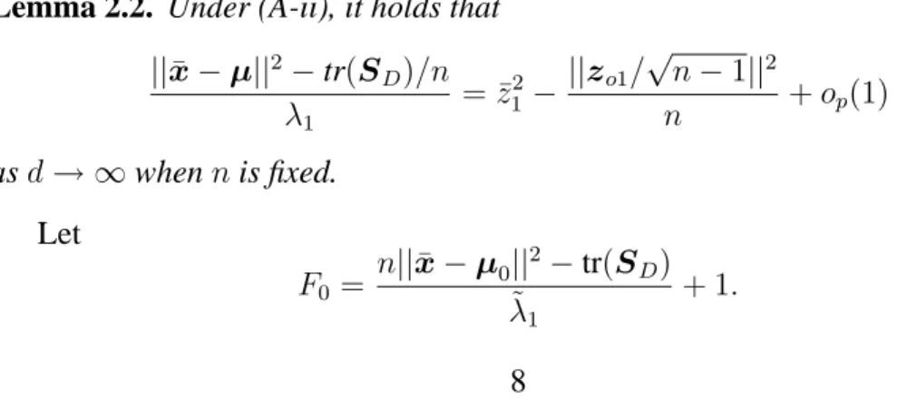
The findings were obtained by averaging the outcomes from2000 (=R, say) replications. Under a fixed scenario, suppose that the r-th replication ends with estimates, (λˆ1r, hˆ1r, MSE(ˆs1)r) and (λ˜1r, h˜1r, MSE(˜s1)r) (r = 1, ..., R). Let us simply write λˆ1 = R−1∑Rr=1λˆ1r andλ˜1 = R−1∑Rr=1λ˜1r. We also considered the Monte Carlo variability by var(ˆλ1/λ1) = (R−1)−1∑Rr=1(ˆλ1r−λˆ1)2/λ21and
var(˜λ1/λ1) = (R−1)−1∑Rr=1(˜λ1r−˜λ1)2/λ21. Figure 1 shows the behaviors of
(λˆ1/λ1, λ˜1/λ1) in the left panel and (var(ˆλ1/λ1), var(˜λ1/λ1)) in the right panel
for (a) and (b). We gave the asymptotic variance of λ˜1/λ1 by Var{χ2n−1/(n −
1)}= 0.222from Theorem 2.1 and showed it by the solid line in the right panel. We observed that the sample mean and variance ofλ˜1/λ1 become close to those
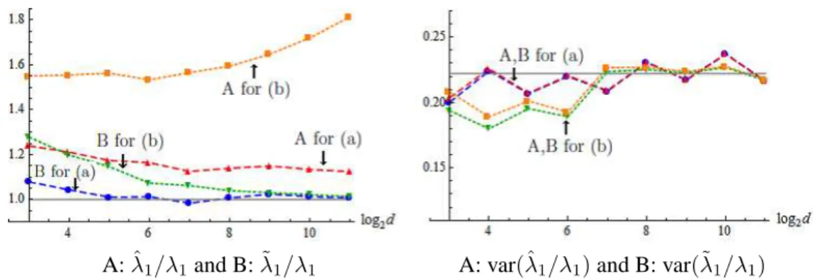
asymptotic values asdincreases. Similarly, we plotted (hˆT1h1, h˜
T
1h1) and (var(ˆh
T
1h1), var(˜h
T
1h1)) in Figure
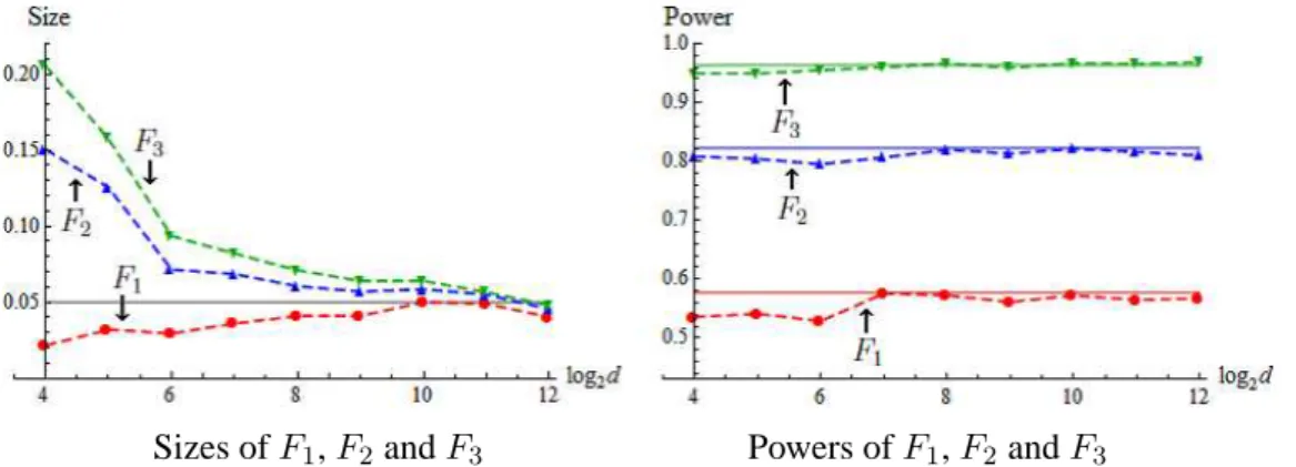
2 and (MSE(ˆs1)/λ1, MSE(˜s1)/λ1) and (var(MSE(ˆs1)/λ1), var(MSE(˜s1)/λ1)) in
Figure 3. From Theorem 3.2, we gave the asymptotic mean of MSE(˜s1)/λ1 by
E(χ2
1/n) = 0.1and showed it by the solid line in the left panel of Figure 3. We
also gave the asymptotic variance of MSE(˜s1)/λ1 by Var(χ21/n) = 0.02 in the
right panel of Figure 3. Throughout, the estimators by the NR method gave good performances both for (a) and (b) when d is large. However, the conventional estimators gave poor performances especially for (b). This is probably because the bias of the conventional estimators,κ/{(n−1)λ1}, is large for (b) compared
to (a). See Proposition 2.1 for the details.
5.2. Equality tests of two covariance matrices
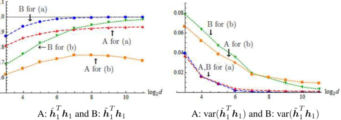
We used computer simulations to study the performance of the test procedures by (4.2) withF1for (4.1),F2for (4.4) andF3for (4.5). We setα = 0.05.
A:ˆλ1/λ1and B:λ˜1/λ1 A: var(ˆλ1/λ1)and B: var(˜λ1/λ1)
Figure 1. The values of A:ˆλ1/λ1and B:λ˜1/λ1are denoted by the dashed lines for
(a) and by the dotted lines for (b) in the left panel. The values of A: var(ˆλ1/λ1)and
B: var(˜λ1/λ1)are denoted by the dashed lines for (a) and by the dotted lines for (b)
in the left panel. The asymptotic variance ofλ˜1/λ1 was given by Var{χ2n−1/(n−
1)}= 0.222and denoted by the solid line in the left panel.
and
Σi =
( Σ
i(1) O2,d−2 Od−2,2 Σi(2)
)
, i= 1,2, (5.1)
whereOk,lis thek×lzero matrix,Σ1(1) =diag(d3/4, d1/2)andΣ1(2) = (0.3|s−t|).
When considered the alternative hypotheses, we set
Σ2(1)=
(
1/√2 1/√2 1/√2 −1/√2
)
diag(3d3/4,1.5d1/2)
(
1/√2 1/√2 1/√2 −1/√2
)
(5.2)
andΣ2(2)= 1.5(0.3|s−t|). Note thatλ1(2)/λ1(1)= 3,κ2/κ1 = 1.5andhT
1(1)h1(2)=
1/√2. Also, note that (A-i) to (A-iii) hold for eachπi. Leth= max{|hT1(1)h1(2)|,
|hT1(1)h1(2)|−1} and γ = max{κ1/κ2, κ2/κ1}. From Lemmas 2.1 and 4.1, it
holds that ˜h = h+op(1) andγ˜ = γ +op(1). Thus, from Corollary 4.1, The-orems 4.1 and 4.2, we obtained the asymptotic powers of F1, F2 and F3 with
(˜h∗,γ˜∗) = (h−1, γ−1)as follows:
Power(F1) =P
{
(λ1(1)/λ1(2))f /∈[{Fν2,ν1(α/2)}
−1, F
ν1,ν2(α/2)]
}
= 0.577,
Power(F2) =P
{
h−1(λ1(1)/λ1(2))f /∈[{Fν2,ν1(α/2)}
−1, F
ν1,ν2(α/2)]
}
= 0.823 and Power(F3) =P
{
γ−1h−1(λ1(1)/λ1(2))f /∈[{Fν2,ν1(α/2)}
−1, F
ν1,ν2(α/2)]
}
A:hˆT
1h1 and B:h˜
T
1h1 A: var(ˆh
T
1h1)and B: var(˜h
T
1h1)
Figure 2. The values of A:hˆT1h1and B:h˜T1h1are denoted by the dashed lines for
(a) and by the dotted lines for (b) in the left panel. The values of A: var(ˆhT1h1)
and B: var(˜hT1h1)are denoted by the dashed lines for (a) and by the dotted lines
for (b) in the right panel.
A: MSE(ˆs1)/λ1and B: MSE(˜s1)/λ1 A: var(MSE(ˆs1)/λ1) and B: var(MSE(˜s1)/λ1)
Figure 3. The values of A: MSE(ˆs1)/λ1 and B: MSE(˜s1)/λ1 are denoted by the
dashed lines for (a) and by the dotted lines for (b) in the left panel. The values of A: var(MSE(ˆs1)/λ1) and B: var(MSE(˜s1)/λ1) are denoted by the dashed lines
for (a) and by the dotted lines for (b) in the right panel. The asymptotic mean and variance of MSE(˜s1)/λ1 were given by E(χ21/n) = 0.1 and Var(χ21/n) = 0.02
Sizes ofF1,F2andF3 Powers ofF1,F2andF3
Figure 4. The values ofαare denoted by the dashed lines in the left panel and the values of1−βare denoted by the dashed lines in the right panel forF1,F2andF3.
The asymptotic powers were given by Power(F1) = 0.577, Power(F2) = 0.823
and Power(F3) = 0.963which were denoted by the solid lines in the right panel.
wheref denotes a random variable distributed as F distribution with degrees of freedom,ν1 andν2. Note that Power(F2)and Power(F3)give lower bounds of the
asymptotic powers when˜h∗ =h−1 andγ˜∗ =γ−1.
In Figure 4, we summarized the findings obtained by averaging the outcomes from 4000 (= R, say) replications. Here, the first 2000 replications were gen-erated by setting Σ2 = Σ1 as in (5.1) and the last 2000 replications were gen-erated by setting Σ2 as in (5.2). Let Fir (i = 1,2,3) be the rth observation of Fi for r = 1, ...,4000. We defined Pr = 1 (or 0) when H0 was falsely
rejected (or not) for r = 1, ...,2000, and Ha was falsely rejected (or not) for
r = 2001, ...,4000. We defined α = (R/2)−1∑R/2
r=1Pr to estimate the size and
1−β = 1−(R/2)−1∑R
r=R/2+1Pr to estimate the power. Their standard
devi-ations are less than0.011. Whend is not sufficiently large, we observed that the sizes of F2 andF3 are quite higher than α. This is probably because ˜h∗ (≥ 1) andγ˜∗ (≥ 1)are much larger than 1. Actually, the sizes became close toα asd increases. Whendis large,F3 gave excellent performances both for the size and
power.
Appendix A.
Proof of Proposition 2.1. We assumeµ=0without loss of generality. We write that XTX = ∑i∗
s=1λszszTs +
∑d
s=i∗+1λszsz
T
s fori∗ = 1whenn is fixed, and for some fixed i∗(≥ 1)when n → ∞. Here, by using Markov’s inequality, for anyτ > 0, under (A-ii) and (A-iii), we have that
P{
n
∑
j=1
( ∑d
s=i∗+1
λs(z2
sj−1)
nλ1
)2
> τ}≤
∑d
r,s≥2λrλsE{(z2rk−1)(zsk2 −1)}
τ nλ2
1 →
0
and P{
n
∑
j̸=j′
( ∑d
s=i∗+1
λszsjzsj′
nλ1
)2
> τ}≤ δi∗
τ λ2 1
→0 (A.1)
as d → ∞ either when n is fixed or n → ∞. Note that ∑n
j=1e4j ≤ 1 and
∑n
j̸=j′e2je2j′ ≤1. Then, under (A-ii) and (A-iii), we have that
n ∑ j=1
e2j
d
∑
s=i∗+1
λs(zsj2 −1)
nλ1
≤
{∑n
j=1
e4j}1/2{
n
∑
j=1
( ∑d
s=i∗+1
λs(zsj2 −1)
nλ1
)2}1/2
=op(1) and
n
∑
j̸=j′
ejej′
d
∑
s=i∗+1
λszsjzsj′
nλ1
≤
{∑n
j̸=j′
e2je2j′
}1/2{∑n
j̸=j′
( ∑d
s=i∗+1
λszsjzsj′
nλ1
)2}1/2
=op(1)
asd→ ∞either whennis fixed orn→ ∞. Thus, we claim that
eTn X
TX
(n−1)λ1
en=eTn
∑i∗
s=1λszszTs (n−1)λ1
en+
κ
(n−1)λ1
+op(1) (A.2)
from the fact that∑d
s=i∗+1λs/{(n−1)λ1}=κ/{(n−1)λ1}+o(1)whenn → ∞.
Note that eTnPn = eTn andPnzs = zos for all s. Also, note that zToszos′/n =
op(1)fors ̸=s′ asn→ ∞from the fact thatE{(zT
oszos′/n)2}=o(1)asn → ∞.
Then, by noting that P(limd→∞||zo1|| ̸= 0) = 1, lim infd→∞λ1/λ2 > 1 and zTo11n = 0, it holds that
max
en {
eTn
∑i∗
s=1λszszTs (n−1)λ1
en}= max
en {
eTn
∑i∗
s=1λszoszTos (n−1)λ1
en}
=||zo1/
√
asd→ ∞either whennis fixed orn → ∞. Note thatuˆT11n = 0anduˆT
1Pn= ˆuT1
whenSD ̸=O. Then, from (A.2), (A.3) andPnXTXPn/(n−1) =SD, under (A-ii) and (A-iii), we have that
ˆ
uT1 SD
λ1
ˆ
u1 = ˆuT1
XTX
(n−1)λ1
ˆ
u1 =||zo1/
√
n−1||2+ κ (n−1)λ1
+op(1) (A.4)
asd→ ∞either whennis fixed orn→ ∞. It concludes the result. ✷
Proof of Lemma 2.1. By using Markov’s inequality, for anyτ > 0, under (A-ii) and (A-iii), we have that
P{(
d
∑
s=2
λs{||zos||2−(n−1)} (n−1)λ1
)2
> τ}
=P{(
d
∑
s=2
λs{(n−1)∑kn=1(zsk2 −1)/n−
∑n
k̸=k′zskzsk′/n}
(n−1)λ1
)2
> τ}
=O{
∑d
r,s≥2λrλsE{(zrk2 −1)(z2sk−1)}
nλ2 1
}
+O{δ1/(nλ1)2} →0
as d → ∞ either when n is fixed or n → ∞. Thus it holds that tr(SD)/λ1 =
κ/λ1+||zo1/√n−1||2+op(1)from the fact that tr(SD) = λ1||zo1||2/(n−1) +
∑d
s=2λs||zos||2/(n−1). Then, from Proposition 2.1 andlim infd→∞κ/λ1 > 0,
we can claim the results. ✷
Proof of Theorem 2.1. Whenn → ∞, we can claim the results from Theorems 4.1, 4.2 and Corollary 4.1 in Yata and Aoshima (2013). Whennis fixed, we can claim the results from Theorem 3.1 and Corollary 3.1 in Ishii et al. (2014). ✷
Proof of Theorem 2.2. From Theorem 2.1 and Lemma 2.1, under (A-i) to (A-iii), it holds that
P( λ1
tr(Σ) ∈
[ (n−1)˜λ1
bκ˜+ (n−1)˜λ1
, (n−1)˜λ1 aκ˜+ (n−1)˜λ1
])
=P( (n−1)˜λ1 bκ˜+ (n−1)˜λ1
≤ λ1
tr(Σ) ≤
(n−1)˜λ1
aκ˜+ (n−1)˜λ1
)
=P( aκ˜
(n−1)˜λ1
≤ λκ
1 ≤
b˜κ
(n−1)˜λ1
)
=P(a≤(n−1)λ˜1κ
λ1˜κ ≤
b)
asd→ ∞whennis fixed. It concludes the result. ✷
Proof of Lemma 2.2. We write that
n||x¯−µ||2−tr(SD) = d
∑
s=1
λs
(
nz¯s2− n
∑
j=1
(zsj −z¯s)2
n−1
)
.
Then, from (A.1) andnz¯2
s −
∑n
j=1(zsj −z¯s)2/(n−1) =
∑n
j̸=j′zsjzsj′/(n−1)
for alls, under (A-ii), we have that
{||x¯−µ||2−tr(SD)/n}/λ1 = ¯zs2− ||zo1/
√
n−1||2/n+op(1)
asd→ ∞whennis fixed. It concludes the result. ✷
Proof of Theorem 2.3. Under (A-i), we note that z¯1 and zo1 are independent,
and nz¯2
1 is distributed as χ21. Then, from Theorem 2.1 and Lemma 2.2, we can
conclude the result. ✷
Proofs of Lemmas 3.1 and 3.2. We note that ||zo1||2/n = 1 +op(1)asn → ∞.
From (A.4), under (A-ii) and (A-iii), we have that
ˆ
uT1zo1/||zo1||= 1 +op(1) (A.5)
asd → ∞either whenn is fixed orn → ∞, so thatuˆT1zo1 =||zo1||+op(n1/2). Thus, we can claim the result of Lemma 3.2. On the other hand, with the help of Proposition 2.1, under (A-ii) and (A-iii), it holds that from (A.5)
hT1hˆ1 =
hT1(X −X)ˆu1
{(n−1)ˆλ1}1/2
= λ
1/2 1 zTo1uˆ1
{(n−1)ˆλ1}1/2
= ||zo1||+op(n
1/2)
{||zo1||2 +κ/λ
1+op(n)}1/2
= 1
{1 +κ/(λ1||zo1||2)}1/2
+op(1)
as d → ∞either when n is fixed orn → ∞. It concludes the result of Lemma
3.1. ✷
Proof of Theorem 3.1. With the help of Theorem 2.1, under (A-ii) and (A-iii), we have that from (A.5)
hT1h˜1 =
hT1(X −X)ˆu1 {(n−1)˜λ1}1/2
= ||zo1||+op(n
1/2)
{||zo1||2+op(n)}1/2
asd→ ∞either whennis fixed orn→ ∞. It concludes the result. ✷
Proof of Theorem 3.2. By combing Theorem 2.1 with Lemma 3.2, under (A-ii) and (A-iii), we have that
˜
s1j/
√
λ1 = ˆu1j
√
(n−1)˜λ1/λ1 = ˆu1j||zo1||+op(1) =zo1j+op(1) asd→ ∞whennis fixed. By noting thatzo1j =z1j −z¯1 andz¯1 is distributed as
N(0,1/n)under (A-i), we have the results. ✷
Proof of Corollary 4.1. From Theorem 2.1, the result is obtained
straightfor-wardly. ✷
Proof of Lemma 4.1. Let Zi = [z1(i), ...,zd(i)]T be a sphered data matrix of πi fori = 1,2, wherezj(i) = (zj1(i), ..., zjni(i))
T. We assumeµ
1 =µ2 =0without
loss of generality. Letβst = (λs(1)λt(2))1/2hTs(1)ht(2) for alls, t. Leti⋆ be a fixed constant such that∑d
s=i⋆+1λ
2
s(j)/λ21(j) = o(1) asd → ∞forj = 1,2. Note that
i⋆ exists under (A-ii) for eachπi. We write that
XT1X2 =
∑
s,t≤i⋆
βstzs(1)zTt(2)+
d
∑
s,t≥i⋆+1
βstzs(1)zTt(2)
+ d
∑
s=i⋆+1
i⋆ ∑
t=1
βstzs(1)zTt(2)+
i⋆ ∑
s=1
d
∑
t=i⋆+1
βstzs(1)zTt(2).
Note that
E{(
d
∑
s=i⋆+1
i⋆ ∑
t=1
βstzsj(1)ztj′(2) )2}
=tr( d
∑
s=i⋆+1
λs(1)hs(1)hTs(1)
i⋆ ∑
t=1
λt(2)ht(2)hTt(2)
)
≤i⋆λi⋆+1(1)λ1(2)
for allj, j′. Also, note that
E{(
d
∑
s,t≥i⋆+1
βstzsj(1)ztj′(2) )2}
=tr
( ∑d
s=i⋆+1
λs(1)hs(1)hTs(1)
d
∑
t=i⋆+1
λt(2)ht(2)hTt(2)
)
≤(
d
∑
s=i⋆+1
λ2s(1)
d
∑
t=i⋆+1
for all j, j′. Then, by using Markov’s inequality, for any τ > 0, under (A-ii) for eachπi, we have that
P{ n1 ∑ j=1 n2 ∑
j′=1
( ∑d
s=i⋆+1
i⋆ ∑
t=1
βstzsj(1)ztj′(2)
(n1n2λ1(1)λ1(2))1/2
)2
> τ}→0,
P{ n1 ∑ j=1 n2 ∑
j′=1 (∑i⋆
s=1
d
∑
t=i⋆+1
βstzsj(1)ztj′(2)
(n1n2λ1(1)λ1(2))1/2
)2
> τ}→0
andP{
n1
∑
j=1
n2
∑
j′=1
( ∑d
s,t≥i⋆+1
βstzsj(1)ztj′(2)
(n1n2λ1(1)λ1(2))1/2
)2
> τ}→0
asd→ ∞either whenniis fixed orni → ∞fori= 1,2. Hence, similar to (A.2), it holds that
eTn1XT1X2en2
(ν1ν2λ1(1)λ1(2))1/2
= e T n1
∑
s,t≤i⋆βstzs(1)z
T t(2)en2
(ν1ν2λ1(1)λ1(2))1/2
+op(1).
Note that eTn
iPni = e
T
ni and Pniz1(i) = zo1(i) for i = 1,2, where zo1(i) =
z1(i)− (¯z1(i), ...,z¯1(i))T and z¯1(i) = n−i 1
∑ni
k=1z1k(i). Also, note that XiPni =
(Xi −Xi)for i = 1,2, whereXi = [¯xi, ...,x¯i]and x¯i = ∑jn=1i xj(i)/ni. Let ˆ
u1(i) be the first (unit) eigenvector of(Xi−Xi)T(Xi−Xi)fori = 1,2. Note thatuˆT1(i)Pni = ˆu1(Ti)when(Xi−Xi)T(X
i−Xi)̸=Ofori= 1,2. Then, under (A-ii) for eachπi, we have that
ˆ
uT1(1)(X1−X1)T(X
2−X2)ˆu1(2)
(ν1ν2λ1(1)λ1(2))1/2
= uˆ T
1(1)
∑
s,t≤i⋆βstzos(1)z
T
ot(2)uˆ1(2)
(ν1ν2λ1(1)λ1(2))1/2
+op(1) (A.6) as d → ∞either when ni is fixed or ni → ∞for i = 1,2. Note that h˜1(i) =
{νiλ˜1(i)}−1/2(Xi −Xi)ˆu1(i)fori= 1,2. Also, note thatzTos(i)zos′(i)/ni =op(1)
(s̸=s′)whenn
i → ∞fori= 1,2. Then, by combining (A.6) with Theorem 2.1
and (A.5), we can claim the result. ✷
Proofs of Theorems 4.1 and 4.2. By combining Theorem 2.1, Lemmas 2.1 and
4.1, we can claim the results. ✷
Acknowledgements
Young Scientists (B), Japan Society for the Promotion of Science (JSPS), under Contract Number 26800078. The research of the third author was partially sup-ported by Grants-in-Aid for Scientific Research (B) and Challenging Exploratory Research, JSPS, under Contract Numbers 22300094 and 26540010.
References
Ahn, J., Marron, J.S., Muller, K.M., Chi, Y.-Y., 2007. The high-dimension, low-sample-size geometric representation holds under mild conditions. Biometrika 94, 760-766.
Aoshima, M., Yata, K., 2011. Two-stage procedures for high-dimensional data. Sequential Anal. (Editor’s special invited paper) 30, 356-399.
Aoshima, M., Yata, K., 2015. Asymptotic normality for inference on multisam-ple, high-dimensional mean vectors under mild conditions. Methodol. Comput. Appl. Probab. 17, 419-439.
Bai, Z., Saranadasa, H., 1996. Effect of high dimension: By an example of a two sample problem. Statistica Sinica 6, 311-329.
Chen, S.X., Qin, Y.-L., 2010. A two-sample test for high-dimensional data with applications to gene-set testing. Ann. Statist. 38, 808-835.
Hall, P., Marron, J.S., Neeman, A., 2005. Geometric representation of high di-mension, low sample size data. J. R. Statist. Soc. B 67, 427-444.
Ishii, A., Yata, K., Aoshima, M., 2014. Asymptotic distribution of the largest eigenvalue via geometric representations of high-dimension, low-sample-size data. Sri Lankan J. Appl. Statist., Special Issue: Modern Statistical Methodolo-gies in the Cutting Edge of Science (ed. Mukhopadhyay, N.), 81-94.
Jeffery, I.B., Higgins, D.G., Culhane, A.C., 2006. Comparison and evaluation of methods for generating differentially expressed gene lists from microarray data. BMC Bioinformatics 7, 359.
Jung, S., Marron, J.S., 2009. PCA consistency in high dimension, low sample size context. Ann. Statist. 37, 4104-4130.
Shipp, M.A., Ross, K.N., Tamayo, P., Weng, A.P., Kutok, J.L., Aguiar R.C., Gaasenbeek, M., Angelo, M., Reich, M., Pinkus, G.S., Ray, T.S., Koval, M.A., Last, K.W., Norton, A., Lister, T.A., Mesirov, J., Neuberg, D.S., Lander, E.S., Aster, J.C., Golub, T.R., 2002. Diffuse large B-cell lymphoma outcome pre-diction by gene-expression profiling and supervised machine learning. Nature Medicine 8, 68-74.
Singh, D., Febbo, P.G., Ross, K., Jackson, D.G., Manola, J., Ladd, C., Tamayo, P., Renshaw, A.A., D’Amico, A.V., Richie, J.P., Lander, E.S., Loda, M., Kantoff, P.W., Golub, T.R., Sellers, W.R., 2002. Gene expression correlates of clinical prostate cancer behavior. Cancer Cell 1, 203-209.
Srivastava, M.S., Yanagihara, H., 2010. Testing the equality of several covariance matrices with fewer observations than the dimension. J. Multivariate Anal. 101, 1319-1329.
Yata, K., Aoshima, M., 2009. PCA consistency for non-Gaussian data in high dimension, low sample size context. Commun. Statist. Theory Methods, Special Issue Honoring Zacks, S. (ed. Mukhopadhyay, N.) 38, 2634-2652.
Yata, K., Aoshima, M., 2010. Effective PCA for high-dimension, low-sample-size data with singular value decomposition of cross data matrix. J. Multivariate Anal. 101, 2060-2077.
Yata, K., Aoshima, M., 2012. Effective PCA for high-dimension, low-sample-size data with noise reduction via geometric representations. J. Multivariate Anal. 105, 193-215.