Building Statistical Hypothesis Tests for Fuzzy Data and Their Applications to
Decision Making
Pei-Chun LIN
Graduate School of Information, Production and Systems Waseda University
April 2013
Title Page i
Contents ii
Abstracts v
Citations to Previous Publish Work x
List of Figures xi
List of Tables xii
Acknowledgements xiv
Dedications xvi
1 Introduction 1
1.1 Background . . . 1
1.2 Motivation and Objective . . . 3
1.3 Research Framework . . . 4
1.4 Structure of the Thesis . . . 4
2 Some Basic Theoretical Concepts 8 2.1 Fuzzy Numbers . . . 8
2.2 Fuzzy Statistic Analysis . . . 10
2.3 Nonparametric Statistical Method . . . 10
2.3.1 Kolmogorov-Smirnov Two-Sample Test . . . 10
CONTENTS
3 Kolmogorov-Smirnov Two Sample Test with Continuous Fuzzy Data 13
3.1 Introduction . . . 13
3.2 Preliminary Preparation . . . 14
3.3 Kolmogorov-Smirnov Two-Sample Test with Continuous Fuzzy Data . . 15
3.3.1 Empirical distribution function with continuous fuzzy data . . . 15
3.3.2 Kolmogorov-Smirnov two-sample test with continuous fuzzy data 19 3.4 Empirical Studies . . . 20
3.5 Summary of Chapter 3 . . . 26
4 Identifying the Distribution Differences of Fuzzy Data Based on a Nonparametric Statistical Method 28 4.1 Introduction and Literature Review . . . 28
4.2 Identifying the Distribution Difference of Fuzzy Data Based on a Non- parametric Statistical Method . . . 30
4.2.1 Realization of a Continuous Fuzzy Data . . . 30
4.2.2 Identifying the Distribution Difference of Fuzzy Data Based on a Nonparametric Statistical Method . . . 35
4.3 Empirical Studies . . . 37
4.4 Comparison of Each Methods . . . 42
4.5 Summary of Chapter 4 . . . 46
5 Risk Assessment of a Portfolio Selection Model Based on a Fuzzy Statistical Test 47 5.1 Introduction . . . 47
5.2 Notations and Preliminary Definitions . . . 49
5.2.1 Statistical Analysis . . . 51
5.2.2 Markowitz’s Portfolio Selection Model . . . 52
5.3 Fuzzy Statistical Test on the Portfolio Selection Model . . . 53
5.3.1 Portfolio Selection Model with Interval Values . . . 54
5.3.2 Fuzzy Statistical Test for the Portfolio Selection Model . . . 56
5.3.3 Procedure of Solving Portfolio Selection Model with Interval Values 57 5.4 Empirical Studies . . . 58
5.5 Summary of Chapter 5 . . . 64
5.5.1 Discussion . . . 64
5.5.2 Conclusions . . . 66
6 A Parametric Assessment Approach to Solving Facility Location Prob- lems with Fuzzy Demands 68 6.1 Introduction and Literature Review . . . 68
6.2 Preliminary Definitions . . . 71
6.3 Problem Statements . . . 74
6.4 Empirical Study . . . 80
6.5 Summary of Chapter 6 . . . 86
6.5.1 Comparison . . . 86
6.5.2 Conclusions . . . 88
7 Conclusions and Future Work 90 7.1 Conclusions . . . 90
7.2 Future Work . . . 92
Bibliography 94 Appendix of Tables 100 Appendix A Kolmogorov-Smirnov Two-Sample Statistic . . . 100
List of Publications 101
Abstract
In conventional statistical methods, hypothesis tests play a fundamental role in making decisions. But in real-world applications, sometimes vague information is given such as in linguistic expression like ”parts of the product are good.” It is not easy to deal with such linguistic expressions in statistical terms. Therefore, we must establish some statistical methods to deal with those vague data.
A statistical hypothesis test plays a pivotal role in social science research.
This test analyzes data in either a controlled experiment or an observational study (not controlled) for making decisions. Relevant null hypothesis H0 and alternative hypothesis H1 are stated the first step in testing process.
We should decide which test should be used and select a significance levelα for making decision. Popular significance levels are 10%, 5%, 1%, 0.5%, and 0.1%. Usually, whenαis chosen, we have the (1−α) confidence interval for the parameter which we want to estimate. We do not reject theH0 when the statistic value is included in (1−α) confidence interval. The statistic test results under a pre-specified significance level can help us to decide whether experimental results contain enough information to cast doubt on conventional perception.
The objective of this thesis is to create a new type of fuzzy hypoth- esis test that can deal with continuous fuzzy data. In addition, we also explain various statistically significant results in risk and error assessment applications.
In the thesis, extending conventional statistical method, we build up new statistical methods that can deal with fuzzy numbers. We call this type of statistical method as ”fuzzy statistics.” Following Zadeh’s concepts and definitions, we use fuzzy set theory to deal with the fuzzy statistics
fuzzy data. In addition, this thesis illustrates two real-life applications of fuzzy statistical test. The structure of the thesis is summarized as follows:
Chapter 1 of this thesis provides the background and motivation for the study as well as the objective of this thesis. We also describe the framework and structure of this thesis.
Chapter 2 provides some preliminary concepts and methods, including fuzzy numbers, fuzzy statistical analysis and a nonparametric statistical method.
In chapter 3, we extend the Kolmogorov-Smirnov (K-S) two-sample test for continuous fuzzy data. The K-S two-sample test is a goodness-of-fit test that is used to determine whether two underlying one-dimensional probabil- ity distributions differ. To find the statistical value of a K-S two-sample test, we calculate the cumulative distribution function by means of the empirical distribution function. In this chapter, we define a new function called the weight function (denoted as WF) that can defuzzify the continuous fuzzy data into real numbers. Thus, the empirical distribution function can be estimated by using those real numbers obtained from defuzzification. In this chapter, we treat three types of fuzzy data in empirical studies. That is, we handle interval values, triangular fuzzy data or trapezoidal fuzzy data in K-S two-sample test. We also provide various significant levels α in this chapter to indicate different results in using K-S two-sample test for con- tinuous fuzzy data. When we used triangular fuzzy data or trapezoidal fuzzy data for K-S two-sample test, we obtained the same statistic value 0.3 in 80% 90%, 95%, 98% and 99% confidence interval in our method and conventional method, where the conventional method used central points to defuzzify the fuzzy data and used this defuzzification in K-S two-sample.
Moreover, when we used interval value for K-S two-sample test, we obtained 0.5 for the statistic value all in 90%, 95%, 98% and 99% confidence interval in our method and we obtained 0.8 for the statistic value that is only in
99% confidence interval in conventional method. It means that we need stronger evidence to confirm the hypothesis when we used interval values for K-S two-sample test in conventional method. Hence, we conclude that our method is more extensive to use K-S two-sample test for continuous fuzzy data that can enable us to judge whether or not two independent samples of continuous fuzzy data come from the same population.
Continuously, we discuss the K-S two-sample test in chapter 4. In this chapter, we compare our proposed method with various methods in iden- tifying the probability distribution differences between two populations of fuzzy data. We derive a function, called realization of a continuous fuzzy data (RF) that can defuzzify continuous fuzzy data. The function RF is different from the function WF in chapter 3. The function WF considers a random variable k, central point and radius but in chapter 4 we consider only the central point and radius. The K-S two-sample test is also used in this chapter for distinguishing two populations of fuzzy data. We illustrated four different defuzzification methods for K-S two-sample test in empirical studies. We proposed a ranking criterion of function RF in this chapter. We said that the fuzzy data are in the same class if they have the same value for defuzzification; otherwise, they are in difference classes. We use func- tion RF to defuzzify the fuzzy data and calculate the empirical distribution function by those defuzzifications. We obtained 0.3 for the statistic value that is in 95% confidence interval in four different defuzzification methods in the experiment and obtained 19 classes in our method (RF method). This number 19 is more than the number of classes, which is 18, in conventional method. Moreover, we have proved that the function WF is a decreasing function. Function WF for K-S two-sample test in chapter 3 does not sat- isfy the ranking criterion which we proposed in this chapter. Hence, it can be concluded that the proposed function RF in chapter 4 is successful in distinguishing two populations of continuous fuzzy data.
In chapter 5, we apply a t-test of fuzzy data to evaluate different risks in a portfolio selection model with fuzzy data. The central points and ra- diuses of fuzzy numbers are used to solve the portfolio selection problem.
central point and radius. We provided different risksk, which is a restric- tion for variance calculated by radius, for investors to make decision. The results of portfolio selection model were interval values composed of central points and radiuses. We obtained the results that we had a stable expected return [5.50, 6.56] because we had the same expected return of radius when k ≥2.81 in our proposed model. Moreover, we obtained a negative value of expected return when k ≤2 in our proposed model. An investor could consider to buy a portfolio when the valuek >2 because we did not want to buy a portfolio with negative expected return in this experiment. Com- paring with other researcher’s method (Zhang implemented the concept of theγ-level to deal with the optimization model), we obtained the expected return [5.41, 6.43] under 95% confidence interval by using the same data in our experiment. The expected return of Zhang’s method is less than our expected return. We concluded that the fuzzy statistical test enables us to evaluate a stable expected return and low-risk investment under different choices ofk.
In chapters 3 to 5, we proposed the statistical methods for fuzzy data. In chapter 6, we describe a real-world application that combines the concept of fuzzy statistics with error assessment. In real-world applications, some- times randomness and fuzziness may coexist. In facility-location problems, vague information included in linguistic should be analyzed. We discussed uncertain demands, called fuzzy demands, in facility location problem. In the facility location model, the parameters of a fuzzy demand are deter- mined by calculating the estimated expected value (EE value) of the fuzzy demand. It was obtained by using estimated parameters of the underly- ing probability distribution function of the fuzzy data. We proposed a defuzzification formula for the fuzzy demand, called the realization of the fuzzy demand (RFD). The RFD formula comprised the upper bound of the fuzzy demand (RF D+) and the lower bound of the fuzzy demand (RF D−).
Moreover, concerning the fuzzy demand, an error assessment itself was eval- uated as mean absolute percentage error of the fuzzy demand (MAPE-FD).
Empirical studies show that we obtained a maximum profit about 5.759 mil- lion NTD. We had less percentage error (27.13%) with respect to distance method, which was proposed by Cheng. If we did not consider MAPE- FD in RFD formula, the percentage error will increase 90.70% more from 27.13% more. But the conventional method obtained a maximum profit about 2.111 million NTD and had 53.40% percentage error with respect to distance method. The results show that, it is better to solve the real- life location problem considering the error assessment (MAPE-FD) in RFD formula.
In the final chapter, we conclude the thesis and suggest several research directions for future work. In this thesis, we have established the statisti- cal test of fuzzy data that is called a fuzzy statistical test. We introduce a concept for ”defuzzifying” fuzzy data into real numbers; that is, we use the central point and radius instead of the fuzzy data. The central point and radius will play a role as statistical characteristics similar to mean and variance. Thus, conventional statistical tests can be applicable to the pa- rameters. To illustrate the efficacy of the proposed method, we introduce two real-life applications: one is a portfolio selection problem, and the other is a facility location problem. Our empirical studies show that we can pro- vide various risk levels and expected returns in portfolio selection problems and it can give more choices for investors to make decisions when they buy exchange currencies. We could also achieve higher profits using the RFD formula in facility location problems. We introduce fuzzy statistical tests to deal with real-life problems in this thesis. We work through problems with interval value and triangular fuzzy data in real-life applications. If we can use fuzzy statistical tests with trapezoidal fuzzy numbers or other types of fuzzy numbers in the future, then this approach will make the proposed method more realistic. Additionally, although we can evaluate our results using a fuzzy statistical test, we also need to consider financial reports, ex- perts’ individual experiences and other factors in the real world for a more well-rounded evaluation.
The contents of Chapter 3 have appeared in the following published papers.
• P.-C. Lin, B. Wu, and J. Watada, Kolmogorov-Smirnov Two Sample Test with Continuous Fuzzy Data,Integrated Uncertainty Management and Applications, Vol.68, pp.175-186, 2010. (Book Chapter)
The contents of Chapter 4 are based on the following published papers.
• P.-C. Lin, J. Watada, and B. Wu, Identifying the Distribution Differ- ence between Two Populations of Fuzzy Data Based on a Nonparamet- ric Statistical Method,IEEJ Transactions on Electronics, Information and Systems, Vol.8, No.6, 2013, to be published.
Large portions of Chapter 5 came from the following published papers.
• P.-C. Lin, J. Watada, and B. Wu, Portfolio Selection Model with In- terval Values Base on Fuzzy Probability Distribution Functions,Inter- national Journal of Innovative Computing, Information and Control, Vol.8, No.8, 2012.
• P.-C. Lin, J. Watada, and B. Wu, Risk Assessment of a Portfolio Se- lection Model Based on a Fuzzy Statistical Test,IEICE Transactions on Information and Systems, Vol.E96-D No.3, 2013, to be published.
Finally, the contents of Chapter 6 have appeared in the following conference paper.
• P.-C. Lin, S. Wang and J. Watada, Decision Making of Facility Lo- cations Based on Fuzzy Probability Distribution Function,The IEEE International Conference on Industrial Engineering and Engineering Management (IEEM 2010), Macao, China, Dec. 7-10, pp.1911-1915, 2010.
List of Figures
1.1 Research Framework . . . 5 3.1 A Triangular Fuzzy Number f(x) with Central Point o and Radius l
Have The Same Area as h(x) . . . 17 4.1 A Trapezoidal Fuzzy Number f(x) with Central Point o and Radius l
Have The Same Area as h(x) . . . 31 5.1 Scatterplot ofmo0,ml0 vs. k . . . 63 6.1 The Potential Facility Sites and Universities in Taipei City . . . 81
3.1 The Price which will be Acceptable by Males and Females . . . 20
3.2 The Weight Values and Classes . . . 21
3.3 The Cumulative Distributions ofXi and Yj . . . 21
3.4 The Price which will be Acceptable by Males and Females . . . 22
3.5 The Weight Values and Classes . . . 23
3.6 The Cumulative Distributions ofXi and Xj . . . 23
3.7 The Price which will be Acceptable by Males and Females . . . 24
3.8 The Weight Values and Classes . . . 25
3.9 The Cumulative Distributions ofXi and Yj . . . 25
3.10 The Results of Hypothesis under Different Significant Level α . . . 27
4.1 The Numbers of E-mails Per Day by Males and Females . . . 37
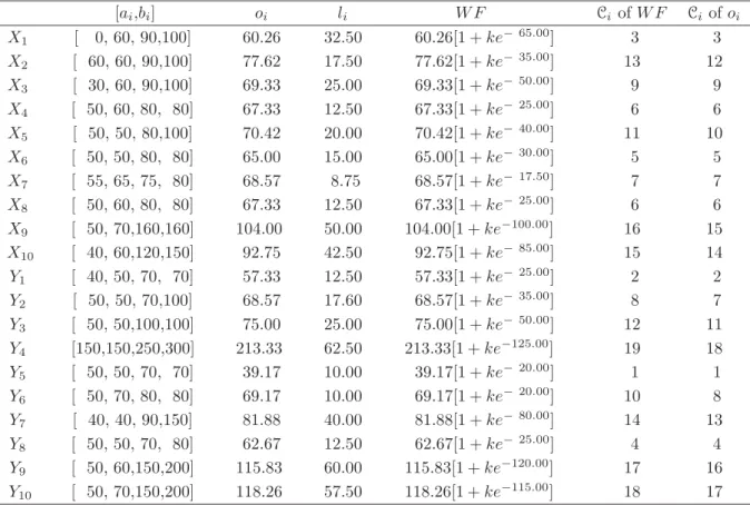
4.2 Values for oi,li,RF and Ci of RF . . . 38
4.3 The Cumulative Distributions ofXi and Yj . . . 38
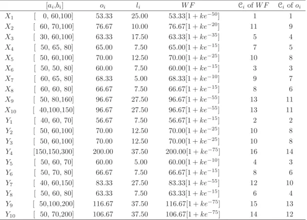
4.4 Values for oi,li,W F and Ci of W F . . . 40
4.5 The Cumulative Distributions ofXi and Yj . . . 40
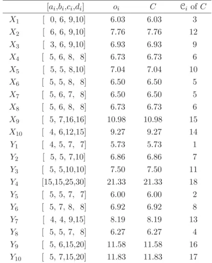
4.6 Values for C, and Ci of C . . . 41
4.7 The Cumulative Distributions ofXi and Yj . . . 41
4.8 Values for ¯xi, ¯yi,RD and Ci ofRD . . . 43
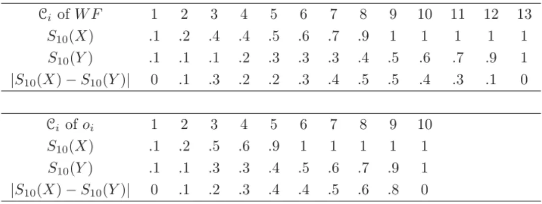
4.9 The Cumulative Distributions ofXi and Yj . . . 43
4.10 Values for RF,Ci ofRF,W F,Ci ofW F,C,Ci of C,RD andCi ofRD 45 4.11 The Results of K-S Two Sample Test in Each Method . . . 45
5.1 Interval Values of Each Exchange Currency . . . 58
5.2 Interval Returns of Each Exchange Currency . . . 59
LIST OF TABLES
5.3 Central Pointo and Radius lof Each Interval Values [A, B] . . . 59
5.4 Parameters of Probability Distribution Functions for Interval Values . . 60
5.5 Expected Values and Variances for Interval Values . . . 60
5.6 Fuzzy Statistical Test for the Results of Model (5.13) with Different Conditions k . . . 61
5.7 The Fuzzy Expected Return with Different Conditions k . . . 62
5.8 Fuzzy Statistical Test for The Results of Model (5.15) and (5.16) with Different Conditions . . . 64
6.1 Triangular Fuzzy Numbers (ak, bk, ck) from Five KFCs. . . 81
6.2 Three Parameters (bk, Lk1, Lk2) of Triangular Fuzzy Numbers from 5 KFCs. 82 6.3 The Probability Distribution Functions for Parameters bj,L1j and L2j. 82 6.4 The EE Value ofbj,L1j andL2j. . . 83
6.5 Decision byt-test . . . 83
6.6 Percentage Error of EE(oj) andEE(lj) . . . 83
6.7 The Parameter Values of RFD . . . 84
6.8 The Fixed Cost, Variable Cost and Capacity for Each Potential Site. . . 85
6.9 The Parameter Values of Distance Method. . . 86
6.10 Solution Comparisons of Location Problem . . . 88
Completing my Ph.D degree is probably the most challenging activity of my life. The best and worst moments of my doctoral journey have been shared with many people. It has been a great privilege to spend four years in the Graduate School of Information, Production and Systems (IPS) at Waseda University. I am indebted to many people for making the time working with me. It’s an unforgettable experience and all members and staffs in Waseda University will always remain dear to me.
Foremost, I would like to express my sincere gratitude to my advisor Professor Junzo Watada for the continuous support of my Ph.D study and research, for his patience, motivation, enthusiasm, and immense knowledge.
His guidance helped me in all the time of research and writing of this thesis.
He has been a steady influence throughout my Ph.D. career.
Besides my advisor, I would like to thank the rest of my thesis committee members, Professor Hee-Hyol Lee, and Professor Tomohiro Murata, for their support, guidance and helpful suggestions.
My sincere thanks also goes to Professor Berlin Wu for providing me many helpful advices and spending his precious time to discuss with me.
To work with him has been a real pleasure to me, with heaps of fun and excitement. He made me feel a friend, which I appreciate from my heart.
I especially thank all members in Watada lab, IPS, Waseda University:
Nureize Bonti Arbaiy, Haydee Rocio Melo Cisneros, Yu-Yi Chu, Hao-Chen Ding, Shinya Imai, Yung-Chin Hsiao, Kim Ikno, Lee-Chuan Lin, You Li, Shamshul Bahar Yaakob, Rozlini Mohamed, Azizul Azhar Bin Ramli, Wen Song, Bo Wang, Shuming Wang, Zhen-Yuan Xu, Jian-Xiong Yang, et al.
They provided many stimulating and entertaining experiences throughout
my Ph.D study. I could not complete my work without invaluable friendly assistance. I owe them my heartfelt appreciation.
I also thank all my friends voluntarily work on Kitakyushu Waseda Taiwanese Student Association-IPS (KWTSA-IPS): Bella Chou, Joy Chu, Perry Chang, Chih-Wei Chen, Zhong-Lun Cai, I-Hsuan Huang, Can Lai, Michael Lee, Wan-Ling Li, Ji-Sheng Peng, Hsin-i Wang, Chan-Long Hsiao, et al. The group could not work well in Kitakyoushu-shi without your help.
Thank you from my heart.
My hearty thanks also go to the members in Kitakyushu Bible Church:
Takemoto Kou sensei, Jessica Kondou, Kondo San, Saori Kondo, Rocky Ayatsuka, Marla Rudd Ayatsuka, Riz Crescini, Anne Larson Crescini, Itou Chiaki, Emily Ark, Junko Fukuda, Nobuko Mitani, et al. They have shel- tered me over the years. They have been like surrogate families, bearing the brunt of the frustrations, and sharing in the joy of the successes. Thank you for just being there for me.
I wish to express my sincere appreciation for the financial support I re- ceived that enable me study and live for years in Japan. Sources included the Scholarship for Young Doctoral Students in Waseda University, Schol- arship for Kitakyushu Science and Research Park (FAIS scholarship) and Honors Scholarship for Privately Financed International Students of Japan Student Services Organization (JASSO). Moreover, I am deeply grateful to Professor Satoshi Goto, the leader of ”Ambient SoC Global COE Program of Waseda University” (GCOE) and all staffs of this program. Without sufficient financial supports from GCOE, it would have been impossible for me to attend those worldwide conferences and high level lectures.
Last but not the last, I would like to thank my love family: my parents provided a loving environment for me. My sister and my younger brother are always unconditionally support me. Their love provided my inspiration and spirituality throughout my life. I owe them a lot.
Finally, I would like to thank Tek-Min Gan. I would not complete this road without your infinite support. I hope that this work makes you proud.
my sister Mei-Ling Lin, and my younger brother Shih-Hao Lin.
1
Introduction
1.1 Background
In social science research, many decisions, evaluations and psychological tests are conducted using surveys and/or questionnaires to seek people’s opinions. It is routine to ask people about their opinions according to binary, multiple-choice questions, but people actually have complex and/or vague thoughts. If we want to understand human thinking in reality, we must create a fuzzy questionnaire (a questionnaire to collect fuzzy data) to seek people’s actual thoughts. However, we seldom use fuzzy surveys (surveys using fuzzy questionnaires) in research studies because it is difficult to find an appropriate statistical method to analyze those fuzzy data.
In real-world applications, sometimes vague information is given when describing data in natural language. Knowing the probability distribution function of fuzzy data plays a pivotal rule in dealing with problems in the real world. Conventional research studies in the past have not recognized the underlying probability distribution function of fuzzy data in their problems. The probability distribution function must be predicted under a specified condition or for a situation given in advance (see (50)). When we want to work with fuzzy data, the underlying probability distribution of the fuzzy data is not known. It is not easy to describe such information in statistical terms. We must establish techniques to handle such information. Following Zadeh (see (83) and (84)), we will use fuzzy set theory and take the concept of fuzzy statistics into consideration.
In conventional statistical methods, nonparametric statistical tests are a distribution- free method in that they make no assumption that the data are drawn from a particular
probability distribution. The two-sample test is one of the most useful nonparametric methods for comparing two samples because it is sensitive to the differences between empirical cumulative distribution functions with regard to both the location and the shape of the two samples. Other nonparametric statistical tests may also be useful (6), such as the median test, the Mann-Whitney test and the parametric t-test. Although these tests are sensitive to differences between two means or medians, they can not de- tect any other type of difference, such as a difference in variance. One of the advantages of two-tailed tests is that such tests consistently reflect all of the types of differences between two distribution functions. The Kolmogorov-Smirnov (K-S) two-sample test is a goodness-of-fit test used to determine whether the two underlying distributions of samples differ.
To manipulate continuous fuzzy data using the K-S two-sample test, we need to cal- culate the empirical distribution function of the continuous fuzzy data first. Therefore, a method is necessary for classifying all of the continuous fuzzy data.
Many research works have proposed various ranking methods to classify fuzzy data.
For instance, Lee-Kwang and Lee (31) proposed a method that derives rankings by considering the overall possibility distributions of fuzzy numbers and provides users with a method for evaluation. Tseng and Klein (68) designed an algorithm to rank any amount of fuzzy numbers. Ota et al. (53) developed a variable axis method (VAM) to decide the complete ordering of fuzzy numbers. Xu and Sasaki (81) proposed a vertex method to calculate the distance between Grey numbers. Lee and You (35) proposed a ranking method that generates possible ranking sequences of given fuzzy numbers.
Kang et al. (21) developed a new fuzzy ranking model based on user preferences.
Hung et al. (19) provided a novel accuracy function to evaluate interval-valued fuzzy information based on intuition. Moreover, Yager (82) proposed a method of ranking fuzzy numbers using a centroid index.
Fundamental statistical measurements such as the mean, the median and the mode are useful for illustrating the characteristics of a sample distribution. More research should focus on the fuzzy statistical aspects of models and their applications in engi- neering, medical and social science. Wu and Cheng (78) identified a model structure through qualitative simulation; Casalinoet al. (5), Esogbue and Song (11), and Wu and Sun (79) discussed the concepts of fuzzy statistics and applied them to social surveys.
Chen and Klein (7) proposed an approach using defuzzification methods for the fuzzy
1.2 Motivation and Objective
MADM. Wu and Tseng (80) used the fuzzy regression method of coefficient estima- tion to analyze the Taiwan monitoring index of economics. In addition, Wu and Sun (79) presented a set of real-life situations in which fuzzy techniques can be naturally reformulated in statistical terms. These studies have addressed various problems us- ing defuzzification techniques to choose the central points of fuzzy numbers. Recently, Wu and Chang (77) evaluated the mean and variance values of interval data based on central point and radius data. Linet al. (40) proposed a new weight function of fuzzy numbers defined by the central point and radius. Moreover, Linet al. (37) proposed a method for recognizing the underlying distribution function using its central point and radius, thereby providing more information about the original fuzzy data. It is more effective to analyze the original fuzzy data. We will take this concept into consideration and integrate it with the concept of fuzzy statistics in this thesis.
1.2 Motivation and Objective
In this thesis, we concentrate our discussion on fuzzy statistical tests. We developed two statistical tests of fuzzy data: a K-S two-sample test of fuzzy data, and at-test of fuzzy data.
Although many papers have discussed the powerful K-S two-sample test (see the discussion in (9), (10), and (60)), these reports have all simulated them under known distributions. No statistical method can distinguish two populations of continuous fuzzy data based on their respective distribution functions. Hence, we use the K-S two- sample test to decide whether the two independent samples of continuous fuzzy data are derived from the same population. We consider a sample of continuous fuzzy data to be a set of data obtained from a single population. Given two different samples of continuous fuzzy data, our goal is to test whether they have been drawn from the same population. This method is useful in various applications, such as industry, engineering, and social surveys.
To use the K-S two-sample test, we need to calculate the empirical distribution function of continuous fuzzy data. We propose a ranking method for fuzzy data in our thesis. This method can classify all continuous fuzzy data and enable us to calculate the empirical distribution function. Although various methods have been proposed to rank fuzzy numbers, all of these methods are based on the concept of a central point.
All of these methods thus ignore some information about the continuous fuzzy data in the calculation. Hence, we propose using two parameters, the central point and radius, to more effectively analyze original fuzzy data.
We still need to make some technical calculations in the processes of developing fuzzy statistical methods. In the real-life applications, we need to find out the prob- ability distribution function of the fuzzy data and each parameter in the probability distribution functions, which enable us to calculate the values in the portfolio selection model and the facility location model. Most studies have not considered any type of probability distribution function with fuzzy data. Moreover, no statistical tests have been applied to examine the results of the proposed models. In view of these weak- nesses, we have developed a t-test to evaluate the results (fuzzy data) of the portfolio selection model. Furthermore, an error assessment, called the mean absolute percentage error of fuzzy demand (MAPE-FD), is proposed in facility location model.
1.3 Research Framework
We show our research framework in Figure1.1.
1.4 Structure of the Thesis
The main work of this dissertation is organized into four relatively independent parts, including (i) The Kolmogorov-Smirnov two-sample test with continuous fuzzy data, (ii) identifying the distribution differences between two populations of fuzzy data based on a nonparametric statistical method, (iii) risk assessment of a portfolio selection model based on a fuzzy statistical test, and (iv) a parametric assessment approach to solving facility location problems with fuzzy demands.
The first part of this thesis provides the background of the study as well as the motivation and objective for this thesis. Moreover, we also provide the framework for and the structure of the thesis.
In Chapter 2, we give some basic theoretical concepts that we will use in the fol- lowing section including fuzzy set theory, fuzzy statistical analysis, and nonparametric statistical methods.
1.4 Structure of the Thesis
WƌŽĚƵĐƚ DĂŶĂŐĞŵĞŶƚ ĨĂĐŝůŝƚLJ ͘͘͘ YƵĞƐƚŝŽŶŶĂŝƌĞ
&ƵnjnjLJĂƚĂ
W ď ďŝůŝ /ŶƚĞƌǀĂů
ĂƚĂ
dƌŝĂŶŐƵůĂƌ
&ƵnjnjLJĂƚĂ
dƌĂƉĞnjŽŝĚ
&ƵnjnjLJĂƚĂ
WƌŽďĂďŝůŝƚLJ ŝƐƚƌŝďƵƚŝŽŶ
&ƵŶĐƚŝŽŶ
<ŽůŵŽŐŽƌŽǀͲ^ŵŝƌŶŽǀdǁŽ^ĂŵƉůĞdĞƐƚ
/ĚĞŶƚŝĨLJƚŚĞŝƐƚƌŝďƵƚŝŽŶŝĨĨĞƌĞŶĐĞ ƉƉůŝĐĂƚŝŽŶ
WŽƌƚĨŽůŝŽ^ĞůĞĐƚŝŽŶWƌŽďůĞŵƐ &ĂĐŝůŝƚLJ>ŽĐĂƚŝŽŶWƌŽďůĞŵƐ
dͲdĞƐƚ DW
ZŝƐŬƐƐĞƐƐŵĞŶƚ WĂƌĂŵĞƚƌŝĐƐƐĞƐƐŵĞŶƚ
dͲdĞƐƚ DW
In chapter 3, a nonparametric statistical method is discussed. We introduce the K-S two-sample test with continuous fuzzy data. The K-S two-sample test is a goodness-of- fit test that is used to determine whether two underlying one-dimensional probability distributions differ. To find the statistical pivot of a K-S two-sample test, we calculate the cumulative function by means of the empirical distribution function. When we address fuzzy data, it is essential to know how to find the empirical distribution function for continuous fuzzy data. In this chapter, we define a new function, the weight function, that can be used to address continuous fuzzy data. Moreover, we can divide samples into different classes. The cumulative function can be calculated with those divided data. The paper explains that the K-S two-sample test for continuous fuzzy data can make it possible to judge whether two independent samples of continuous fuzzy data come from the same population. The results show that it is realistic and reasonable to use the K-S two-sample test with continuous fuzzy data in social science research.
In chapter 4, we continue to introduce a nonparametric statistical method for ana- lyzing fuzzy data. Nonparametric statistical tests are distribution-free methods without any assumption that data are drawn from a particular probability distribution. In this chapter, to identify the distribution differences between two populations of fuzzy data, we derive a function that can describe continuous fuzzy data. The function is different from the weight function in chapter 3. The K-S two-sample test is also used in this chapter for distinguishing two populations of fuzzy data. Empirical studies illustrate that the K-S two-sample test enables us to judge whether two independent samples of continuous fuzzy data are derived from the same population. The results show that the proposed function is successful in distinguishing two populations of continuous fuzzy data and is useful in various applications.
Continuing the discussion, we introduce a statistical test for fuzzy data in Chapter 5. The objective of this chapter is to develop a statistical test that can evaluate the different risks of a portfolio selection model using fuzzy data. The central points and radiuses of fuzzy numbers are used to determine the portfolio selection model, and we statistically evaluate the best return by using a fuzzy statistical test. Empirical studies are presented to illustrate the risk evaluation of the portfolio selection model with interval values. We conclude that the fuzzy statistical test employed enables us to evaluate a stable expected return and low-risk investment with different choices for k,
1.4 Structure of the Thesis
which indicates the risk level. The results of numerical examples show that our method is suitable for short-term investments.
Thus, in chapters 3 to 5, we discuss some statistical methods for fuzzy data. There are still minor problems in dealing with fuzzy data based on fuzzy statistical tests.
We introduce error assessment in Chapter 6. In real-world applications, sometimes randomness and fuzziness may coexist within a dataset. In facility location problems, data expressed in natural language contain vague information. We discuss uncertainty of the demands in facility location problems. The uncertain demands are referred to as fuzzy demands in this chapter. In the facility location model, the parameters of fuzzy demands are determined by calculating the estimated expected value (EE value) of the fuzzy demand, which is obtained by using estimated parameters of the underlying probability distribution function of the fuzzy data. Moreover, we propose a defuzzification formula for the fuzzy demand called a realization of the fuzzy demand (RFD). The RFD formula consists of the upper bound of the fuzzy demand (RF D+) and the lower bound of the fuzzy demand (RF D−). Moreover, the error of a fuzzy demand is assessed as its mean absolute percentage error of the fuzzy demand (MAPE- FD). Our empirical studies show that we can solve real-life location problems by using the RFD formula and can therefore achieve higher profits in our facility location model in comparison with conventional methods.
In the last section, we conclude chapters 3 to 6 and suggest some research directions for future work.
Some Basic Theoretical Concepts
The focus in this chapter is on some basic theoretical concepts which are necessary for the discussed topic in this thesis.
2.1 Fuzzy Numbers
A fuzzy number is an extension of a regular number in the sense that it does not refer to one single value but rather to a connected set of possible values, where each possible value has its own weight between 0 and 1. This weight is called the membership function. Here, we introduce some definitions with respect to membership functions and fuzzy numbers which we will use in the following chapter.
Definition 2.1 Trapezoidal Membership Function(26)
One class of function frequently used to represent linguistic terms is the class of trapezoidal membership functionsμ(x;a, b, c, d), which are defined as follows:
μA(x;a, b, c, d) =
⎧⎪
⎪⎪
⎪⎪
⎨
⎪⎪
⎪⎪
⎪⎩
0, x < aand x > d x−a
b−a, a≤x≤b 1, b≤x≤c
d−x
d−c, c≤x≤d
.
whereA= [a, b, c, d] is called a trapezoidal fuzzy number.
Especially, whenb=c in Definition 2.1, we get a triangular membership function.
We give a definition of triangular membership function in the following.
2.1 Fuzzy Numbers
Definition 2.2 Triangular Membership Function
Let A = [a, b, c] be a triangular fuzzy number, then its membership function is defined as follows:
μA(x;a, b, c) =
⎧⎪
⎪⎪
⎨
⎪⎪
⎪⎩
0, x < aand x > c x−a
b−a, a≤x≤b c−x
c−b, b≤x≤c
.
Moreover, if a=b and c=d in Definition 2.1, we get a interval value. We give a definition of uniform membership function in the following.
Definition 2.3 Uniform Membership Function
Let A = [a, b] be an interval value, then its membership function is defined as follows:
μA(x;a, b) =
1, a≤x≤b 0, otherwise .
Zadeh (83) proposed fuzzy set theory to deal with the vagueness in data, where membership grade of a fuzzy set is a value between 0 and 1. The following definitions of fuzzy numbers will be used in the whole thesis.
Definition 2.4 (50) Let U be a universal set and C ={C1, C2,· · ·, Cn} be the sub- set of a specified collection of elements in U. For any term or statement X on U, the membership function of {C1, C2,· · · , Cn} is denoted {μ1(X), μ2(X),· · ·, μn(X)}, where μ : U → [0,1] is a real value function. If the domain of the universal set is discrete, then the fuzzy numberx of X can be written as
μU(X) = n i=1
μi(X)ICi(X), (2.1)
whereICi(X) = 1 if x∈Ci, and ICi(X) = 0 if x /∈Ci.
If the domain of the universal set is continuous, then the fuzzy numberxcan be written as
μU(X) =
Ci⊆C
μi(X)ICi(X)dC. (2.2)
Note that, many writings denote a fuzzy number as μU(X) = μ1(X)
C1 +μ2(X)
C2 +· · ·+μn(X) Cn ,
where ”+” stands for ”or”, and ”·” denotes the membershipμi(X) onCi.
2.2 Fuzzy Statistic Analysis
Definition 2.5 Fuzzy Sample Mean (data with interval values) (50)
Let U be a universe set and {Fi = [ai, bi], ai, bi∈ , i= 1,· · · , n} be a sequence of a random fuzzy sample on U. Then, the fuzzy sample mean value is defined as
F¯ = [1 n
n i=1
ai,1 n
n i=1
bi].
Example 2.1 Let F1 = [2,3], F2 = [3,4], F3 = [4,6], F4 = [5,8], and F5 = [3,7] be the starting salary for 5 newly graduated master’s students. Then, the fuzzy sample mean for the starting salary of the graduated students will be
F¯ = [2 + 3 + 4 + 5 + 3
5 ,3 + 4 + 6 + 8 + 7
5 ]
= [3.4,5.6].
2.3 Nonparametric Statistical Method
In this section, we will introduce a conventional statistical test which we will use in the following chapters.
2.3.1 Kolmogorov-Smirnov Two-Sample Test
The Kolmogorov-Smirnov Two-Sample Test (hereafter, K-S two-sample test) is de- signed to evaluate whether two independent samples have been drawn from the same population (or from populations with the same distribution). A two-tailed test is sen- sitive to any kind of difference in the distributions from which the two samples are drawn. A one-tailed test is used to decide whether the sample values in the popula- tion of samples are stochastically larger than the values of the population of the other samples.
To apply the K-S two-sample test, we determine the cumulative frequency distribu- tion for each sample of observations by using the same intervals for both distributions.
Then, for each interval, we subtract one step function from the other. The test focuses on the largest one of these observed deviations.
2.3 Nonparametric Statistical Method
LetSm(X) be the empirical distribution function for one sample of sizem, that is, Sm(X) = 1
m m i=1
IXi≤x, where IXi≤x is the indicator function, equal to 1 if Xi ≤x and equal to 0 otherwise. Let Sn(X) be the empirical distribution function for the other sample of sizen, that is,Sn(X) = 1
n n i=1
IXi≤x. Thus, the K-S two-sample test statistic is
Dm,n =supX[Sm(X)−Sn(X)], (2.3) for a one-tailed test, and it is
Dm,n =supX|Sm(X)−Sn(X)|, (2.4) for a two-tailed test. Note that equation (2.4) uses the absolute value.
In each case, the sampling distribution of Dm,n is known. The probabilities asso- ciated with observed values as large as the observed Dm,n under the null hypothesis (i.e., the two samples have come from the same distribution) are tabled in Reference (47). In fact, there may be two sampling distributions, depending upon whether the test is one-tailed or two-tailed. Notice that for a one-tailed test, we observe Dm,n in the predicted direction using equation (2.3), and for a two-tailed test, we observe the maximum absolute difference Dm,n using equation (2.4), regardless of the direction.
This is because in the one-tailed test,H1 indicates that the population values relating to one of the samples are stochastically larger than the population values relating to the other sample, whereas in the two-tailed test,H1 simply indicates that the two samples are from different populations.
If bothmandnare 25 or less, Appendix TableLI in Reference (63) can be used as a reference to test the null hypothesis against a one-tailed alternative, and Appendix Table LII in Reference (63) can be used as a reference to test the null hypothesis against a two-tailed alternative. These tables give values forDm,n that are significant at various levels. The critical values of the test statistic can be derived if values ofm, n,mnDm,n as well as whether the tests that are one-tailed are known.
When eithermornare larger than 25, Appendix TableLIII in Reference (63) may be used for the K-S two-sample test. To use this table, determine the value of Dm,n for observed data by using the following equation:
K(α) m+n
mn , (2.5)
whereα is the significant level and the value of coefficientK(α) can be found in Table LIII of Reference (63).
Hence, we present the steps of the K-S two-sample test.
Step 1. Arrange both the groups of scores in a cumulative frequency distribution using the same intervals (or classifications) for both distributions. Use as many intervals as possible.
Step 2. Using subtraction, determine the difference between the two-sample cumula- tive distributions.
Step 3. Determine the largest of the differences Dm,n. For a one-tailed test, Dm,n is the largest difference in the predicted direction. For a two-tailed test, Dm,n is the largest difference in either direction.
Step 4. Determine the significance of the observed values Dm,n depending on the sample size and the nature of H1. When m and n are both ≤ 25, Appendix Table LI in Reference (63) is referenced for the one-tailed test, and Appendix Table LII in Reference (63) is referenced for the two-tailed test. In both tables, entry mnDm,n is used. For a two-tailed test when eithermornare larger than 25, Appendix TableLIII in Reference (63) is used. Critical values of Dm,n for any given large values ofm or n may be computed by using the formula (2.5).
Step 5. If the observed value is equal to or greater than that given in the appropriate table for a particular level of significance, H0 may be rejected in favor of H1.
We show a part of Tables of Reference (63) in our Appendix A which we will use in the chapters 3 and 4.
Similar to the K-S one-sample test, the K-S two-sample test focuses on the agree- ment between two cumulative distributions. If the two samples have indeed been drawn from the same population distribution, then the cumulative distributions of both the samples should be expected to be fairly close to each other, inasmuch as they both should show only random derivations from the common population distribution. If the two fuzzy sample cumulative distributions are too far apart at any point, this suggests that the samples come from different populations. Thus, a sufficiently large deviation between the two sample cumulative distributions is evidence to rejectH0.
3
Kolmogorov-Smirnov Two
Sample Test with Continuous Fuzzy Data
3.1 Introduction
The Kolmogorov-Smirnov (K-S) two-sample test is a goodness-of-fit test that is used to determine whether two underlying distributions differ. It is customary to call the K- S two-sample test the Smirnov test (64), while the Kolmogorov test is sometimes called the K-S one-sample test. In this chapter, we discuss only the K-S two-sample test, as our purpose here is to test whether two independent samples have been drawn from the same population. The two-sample test is one of the most useful nonparametric methods for comparing two samples, as it is sensitive to differences in both the location and the shape of the empirical cumulative distribution functions of the two samples. Other tests, such as the median test, the Mann-Whitney test, or the parametric t-test, may also be appropriate (6). However, while these tests are sensitive to differences between two means or medians, they may not detect other types of differences, such as differences in variance. One of the advantages of two-tailed tests is that such tests consistently reflect all types of differences between two distribution functions. Although many papers have discussed the powerful K-S two-sample test (see the discussions in (9), (10), and (60)), these reports have all simulated these tests based on known distributions. However, vague information is sometimes given when describing data in natural language, and the
underlying distribution of the fuzzy data is not known. It can be difficult to put such information into statistical terms; therefore, we must establish techniques to handle such information.
In this chapter, we propose a method of judging whether two continuous fuzzy data samples have been drawn from the same population. We use the K-S two-sample test to address this problem. However, the K-S two-sample test is concerned with real numbers. To manipulate continuous fuzzy data by means of the K-S two-sample test, we must find a method for classifying all of the continuous fuzzy data. Accordingly, we propose some new rules for classifying and ranking continuous fuzzy data. Several ranking methods have previously been proposed for fuzzy numbers; for instance, Chen (8) used the distance between the fuzzy numbers and the comparison data to find the greatest distance. Similar to Kaufmann and Gupta (22), Liou and Wang (41) used a membership function to rank fuzzy numbers. Yager (82) proposed a method of ranking fuzzy numbers using a centroid index. Although there are many ways to rank fuzzy numbers, all the methods that have been used are based on the central point. Any such method will lose some information about continuous fuzzy data. Thus, we use a weight function to rank fuzzy numbers. The weight function includes both the central point and the radius, which can be used to classify all continuous fuzzy data. When we use this information, the K-S two-sample test with continuous fuzzy data can be implemented.
3.2 Preliminary Preparation
First, we give some definitions we will use in this chapter. We determine the fuzzy data as central point and radius by using following definition.
Definition 3.1 Moments and Center of Mass of a Planar Lamina (33)
Let f and g be continuous functions such that f(x) ≥g(x) on [a,b], and consider the planar lamina of uniform density ρ bounded by the graphs of y =f(x), y=g(x), and a≤x≤b.
1. The moments about thex−axis and y−axis are Mx=ρ
b
a
[(f(x) +g(x))
2 ][f(x)−g(x)]dx (3.1)
3.3 Kolmogorov-Smirnov Two-Sample Test with Continuous Fuzzy Data
My =ρ b
a
x[f(x)−g(x)]dx. (3.2)
2. The center of mass (x, y) is given byx= My
m andy= Mx
m , wherem=ρ b
a
[f(x)−g(x)]dx is the mass of the lamina.
Note that in mathematics, a planar lamina is a closed surface of massmand surface densityρ. It can be used to determine moments of inertia, or center of mass.
We also need an definition as follows. We will use it to define our function in this thesis.
Definition 3.2 The Mean Value Theorem for Definite Integrals(14) If f is continuous on [a, b], then there exists some pointsc in [a, b], such that
f(c) = 1 b−a
b
a
f(x)dx.
3.3 Kolmogorov-Smirnov Two-Sample Test with Contin- uous Fuzzy Data
3.3.1 Empirical distribution function with continuous fuzzy data In order to provide the empirical distribution function for continuous fuzzy data, we must classify the continuous fuzzy data. We first define a weight function for con- tinuous fuzzy data, and then use it to pursue a new classification. Thus, the empirical distribution function for the continuous fuzzy data can be found.
In order to correct the data accurately, we use the continuous revising to define the weight function as follows.
Definition 3.3 Weight function for continuous fuzzy data
The weight function of continuous fuzzy dataXi≡(oi, li) is defined as follows:
W Fxi ≡W F(oi, li) =oi[1 +ke−2li],∀i= 1,2,3, . . . (3.3) whereoi is the central point,li is the radius with respect tooi, andk=max(oi+li)− min(oj−lj),∀i, j= 1,2,3. . . .We name kas weight constant.
Property 3.1LetXi = [ai, bi] be an interval value, thenoi= ai+bi
2 , li = bi−ai 2 , and k=max bi−min aj,∀i, j= 1,2,3. . . .
Proof: It is trivial thatoi = ai+bi
2 and li= bi−ai 2 . Therefore, we have
k=max(oi+li)−min(oj−lj)
=max(ai+bi
2 +bi−ai
2 )−min(aj +bj
2 −bj−aj
2 )
=max bi−min aj,∀i, j= 1,2,3. . . .
Property 3.2LetXi = [ai, bi, ci] be triangular fuzzy numbers, thenoi= ai+bi+ci 3 , li = ci−ai
4 , and k=max(ai+ 4bi+ 7ci
12 )−min(7aj+ 4bj +ci
12 ),∀i, j= 1,2,3. . . . Proof: By Definition 3.1, we let ρ= 1 and we can find thatoi = My
m .
When Xi is a triangular fuzzy number, its membership function is denoted as fol- lows:
f(x) =
⎧⎪
⎪⎪
⎨
⎪⎪
⎪⎩
0, x< a and x > c x−a
b−a, a≤x≤b c−x
c−b, b≤x≤c
.
Therefore, My = 1 b
a
xx−a b−adx+ 1
c
b
xc−x
c−bdx= 1
6(c−a)(a+b+c) and m = 1
b
a
x−a b−adx+ 1
c
b
c−x
c−bdx= c−a 2 . Hence,
oi = My m =
1
6(ci−ai)(ai+bi+ci) ci−ai
2
= ai+bi+ci
3 .
Moreover, from Definition 3.2, the mean value theorem for definite integrals (14) enables us to find some pointstin [a,c] such that
(c−a)f(t) = c
a
f(x)dx= c−a 2 . Therefore, f(t) = 1
2,∀t∈[a, c].
In the case where there are two points, say t1 and t2, such that f(t1) =f(t2) = 1
2,∀t1, t2∈[a, c].
3.3 Kolmogorov-Smirnov Two-Sample Test with Continuous Fuzzy Data
u(x)
Membership function f(x) Membership function f(x) h(x)
1
o l
a b x
0 c x
Figure 3.1: A Triangular Fuzzy Number f(x) with Central Pointoand Radiusl Have The Same Area ash(x)
This results in t1= a+b
2 and t2 = b+c 2 .
There also exists a rectangle with the same area as c−a
2 . (See Figure 3.1.) Hence 2l=t2−t1 = c−a
2 , l= c−a 4 .
When we have oi and li, the weight constant kis k=max(oi+li)−min(oj−lj)
=max(ai+bi+ci
3 +ci−ai
4 )−min(ai+bi+ci
3 −ci−ai 4 )
=max(ai+ 4bi+ 7ci
12 )−min(7aj+ 4bj+ci
12 ),∀i, j= 1,2,3. . . Property 3.3 LetXi= [ai, bi, ci, di] be trapezoidal fuzzy numbers, then oi = (ci+di)2−(ai+bi)2+aibi−cidi
3[(ci+di)−(ai+bi)] , li = (ci+di)−(ai+bi)
4 , and k = max(oi + li)−min(oj−lj),∀i, j= 1,2,3. . . .
Proof: By Definition 3.1, we let ρ= 1 and we can find thatoi = My m .
When Xi is a trapezoidal fuzzy number, its membership function is denoted as
follows:
f(x) =
⎧⎪
⎪⎪
⎪⎪
⎨
⎪⎪
⎪⎪
⎪⎩
0, x< aandx > d x−a
b−a, a≤x≤b 1, b≤x≤c
d−x
d−c, c≤x≤d
.
Therefore, My = 1 b
a
xx−a b−adx+ 1
c
b
x1dx+ 1 d
c
xd−x
d−cdx= 1
6[(c+d)2−(a+ b)2+ (ab−cd)] andm= 1
b
a
x−a b−adx+ 1
c
b
1dx+ 1 d
c
d−x
d−cdx= 1
2[(c+d)−(a+b)].
Hence, oi= My
m =
1
6[(c+d)2−(a+b)2+ (ab−cd)]
1
2[(c+d)−(a+b)] = [(c+d)2−(a+b)2+ (ab−cd)]
3[(c+d)−(a+b)] . Moreover, from Definition 3.2, the mean value theorem for definite integrals (14) enables us to find some pointstin [a,d] such that
(d−a)f(t) = d
a
f(x)dx= (c+d)−(a+b)
2 .
Therefore, f(t) = (c+d)(a+b)
2(d−a) ,∀t∈[a, d].
In the case where there are two points, say t1 and t2, such that f(t1) =f(t2) = (c+d)(a+b)
2(d−a) ,∀t1, t2 ∈[a, d].
We can also find a rectangle with the same area as (c+d)(a+b)
2 .
Hence, 2l=t2−t1= (c+d)(a+b)
2 and l= (c+d)(a+b)
4 .
When we have oi and li, the weight constant kis
k=max(oi+li)−min(oj−lj),∀i, j= 1,2,3. . . Definition 3.4 Fuzzy classification
IfW Fxi < W Fxj,∀i=j, we say thatxiandxj are in different classes. In particular, xi is the class before xj. Moreover, if W Fxi =W Fxj,∀i=j, we say thatxi andxj are in the same class.
Definition 3.5 Identical independence of continuous fuzzy data
If W Fxi = W Fxj,∀i = j, we say that xi and xj are identical independent by the choose ofk (weight constant). Otherwise, xi andxj are dependent.
3.3 Kolmogorov-Smirnov Two-Sample Test with Continuous Fuzzy Data
Definition 3.6 Empirical distribution function with continuous fuzzy data Let x1, x2, . . . , xn be n continuous fuzzy data. We can use the weight function (WF) to separate xi into different class ci, which are called Glivenko-Cantelli classes (see discussion in References (13), (15), and (61)). If xi and xj are in different classes, then we say that xi and xj are identically independent for i =j. Moreover, we have the order statistic ofxi (assume that they are in different classes), denoted as
W Fx(1) < W Fx(2) < ... < W Fx(n) (3.4) Hence, the empirical distribution function can be generalized to a set C to obtain an empirical measure indexed byci.
Sn(ci) = 1 n
n i=1
Ici(W Fxi), ci ∈C, (3.5) whereIci is the indicator function denoted by
Ici(W Fxi) =
1, WFxi ∈ci,
0, WFxi ∈/ ci ,∀i= 1,2, . . . n. (3.6) Now, when we have those definitions, we can proceed to study the Kolmogorov- Smirnov two-sample test with continuous fuzzy data.
3.3.2 Kolmogorov-Smirnov two-sample test with continuous fuzzy data
Procedure for using K-S two-sample test for continuous fuzzy data (Two- tailed test) in small samples:
1. Samples: LetXmand Yn be two samples with continuous fuzzy data. Xi has size m andYj has size n. Combining all observations, we haveN =m+npieces of data. A value of the weight functionW F can be found that will let us distribute Xm and Yn into different classes ci (maybe in the same class). The number of classes is less than or equal to N. Moreover, the two empirical distribution functions ofXm and Yn can be found individually.
2. Hypothesis: Two samples have the same distributionH0. 3. Statistics: Dm,n=max|Sm(X)−Sn(X)|.
4. Decision rule: Under significance level α. Appendix A Table I is used.
3.4 Empirical Studies
Example 3.1A Japanese dining hall manager planned to introduce new boxed lunch services and decided to take a survey to investigate what price for a boxed lunch would be acceptable to male and female customers. A sample was randomly selected of 20 customers (10 males and 10 females) who resided around this dining hall in the city of Taipei. The investigator asked them, how many dollars they would be willing to spend (can answer with interval) for a boxed lunch in a Japanese dining hall. The answers are shown in Table3.1.
Table 3.1: The Price which will be Acceptable by Males and Females
Males [60,70] [70,90] [50, 80] [50, 60] [80,100] [70,90] [50,80] [ 50, 70] [65, 95] [50,100]
Females [50,60] [60,70] [80,100] [90,120] [90,100] [55,75] [70,90] [100,120] [80,120] [90,120]
First, we distributed male answers and female answers into different classes. We had to find the weight values and compare them. Moreover, we had to determine which class they belong to. The calculation was done as Table 3.2.
Comparison among W F, results in the following inequality:
W FX4 =W FY1 < W FX8 < W FX3 =W FX7 < W FY6 < W FX1 =W FY2 < W FX10 <
W FX9 < W FX2 = W FX6 = W FY7 < W FX5 = W FY3 < W FY5 < W FY9 < W FY4 = W FY10 < W FY8.
Here, we take k=max bi−min aj = 120−50 = 70,∀i, j= 1,2, . . . ,20.
From the above, we have 13 classes. Now, we went on to find the cumulative distribu- tions of Xi andYj.
From Table 3.3, the test statistic was obtained:
D=max|S10(X)−S10(Y)|= 0.5.
at a significance level α = 0.05, mnD= 10∗10∗(0.5) = 50 <70 (Appendix A Table I). Since the observed value did not exceed the critical value, we did not rejectH0. We conclude that males and females have the same interval of the acceptable price of a boxed lunch.
We use the same data in Table 3.1 and different method to defuzzify the interval values. We denote this method asC method which is a conventional method by using


![Table 4.2: Values for o i , l i , RF and C i of RF [a i ,b i ,c i ,d i ] o i l i RF C i of RF X 1 [ 0, 6, 9,10] 6.03 3.25 6.03 + [1 − e − 3](https://thumb-ap.123doks.com/thumbv2/123deta/9852204.1898125/54.892.183.782.303.816/table-values-rf-c-rf-rf-c-rf.webp)
![Table 4.4: Values for o i , l i , W F and C i of W F [a i ,b i ,c i ,d i ] o i l i W F C i of W F X 1 [ 0, 6, 9,10] 6.03 3.25 6.03[1 + ke − 6](https://thumb-ap.123doks.com/thumbv2/123deta/9852204.1898125/56.892.184.780.304.816/table-values-w-f-c-w-f-w.webp)