コロイド分散系の非平衡定常状態に対する粒子間相 互作用の効果

九州大学学術情報リポジトリ

Kyushu University Institutional Repository

コロイド分散系の非平衡定常状態に対する粒子間相 互作用の効果

井上, 雅郎

https://doi.org/10.15017/1928614

出版情報：Kyushu University, 2017, 博士（理学）, 課程博士 バージョン：

権利関係：

A Thesis Submitted to Kyushu University for the Degree of Doctor of Science

Effects of Interactions between Particles on Nonequilibrium Steady States in

Colloidal Dispersion Systems

Masao Inoue

Department of Physics, Graduate School of

Science, Kyushu University, Japan

Abstract

In this thesis, I clarify effects of interactions between colloidal particles on nonequilibrium steady states in colloidal dispersion systems. I consider a probe particle fixed in a flowing colloidal suspension comprised of hard-sphere colloidal particles and a solvent. Particularly, in the field of microrheology, mechanical properties of a suspension are determined from the relation between the force on probe particles and the flux velocity. In order to examine the effects of interactions between the colloidal particles, I calculate the force exerted by the colloidal parti- cles on the probe particle via numerical calculations using two theoretical methods.

The methods are the time-dependent density functional theory (TDDFT) and the combination of the density functional theory (DFT) with the two-fluid model.

In the first method, assuming that the solvent velocity field is uniform in the whole system, I calculate the force exerted by the colloidal particles on the probe particle via numerical calculations using the TDDFT. By solving numerically the equation of the density field derived from the TDDFT, I obtain the density field of colloidal particles around the probe particle. From the numerical integration of the density field, I calculate the force exerted by the colloidal particles on the hard-sphere probe particle. In order to examine the effects of interactions between the colloidal particles, I compare the results for interacting colloidal particles and those for noninteracting colloidal particles. For small flux velocity, the calculated results show that the force decreases due to the interactions between the colloidal particles. In contrast, for large flux velocity and the large volume fraction of colloids, the force increases due to the interactions.

In the second method, considering the nonuniformity of the solvent velocity

field, I examine the modification of the effect of the interactions obtained in the first

method by this nonuniformity. In order to consider the nonuniform solvent velocity

field disturbed by the colloidal particles, I derive the equations of motion for the

colloidal particles and for the solvent by combining the DFT with the two-fluid

model. Here, I assume that the probe particle is a soft-core particle and the solvent

velocity field is disturbed only by the colloidal particles. Using the expansion

in powers of the volume fraction, I solve the second-order equations numerically

and obtain the density field of the colloidal particles and the nonuniform solvent

velocity field for small volume fractions. The calculated results of the force show

qualitatively the same effect of the interactions between the colloidal particles as

that obtained in the first study using the TDDFT. This means that for small

volume fractions, the effect of the interactions on the force is qualitatively not

modified by the nonuniformity of the solvent velocity field.

Contents

Abstract 1

1 Introduction 4

2 Microrheology 6

2.1 Theoretical study of microrheology . . . . 6

2.1.1 Model system for active microrheology . . . . 7

2.1.2 Motion of probe particle . . . . 8

2.1.3 Density field of colloidal particles . . . . 9

2.1.4 Results of viscosity increment . . . . 12

2.2 Experimental study of microrheology . . . . 13

2.2.1 Preparation . . . . 13

2.2.2 Method . . . . 14

2.2.3 Results . . . . 15

2.3 Summary . . . . 16

3 Two-fluid model 18 3.1 Introduction . . . . 18

3.2 Derivation of equations . . . . 18

3.2.1 Continuity equation and incompressibility condition . . . . . 18

3.2.2 Rayleigh’s variational method . . . . 19

3.2.3 Energy dissipation . . . . 19

3.2.4 Time derivative of free energy . . . . 20

3.2.5 Motion equations at steady states . . . . 21

3.2.6 Approximate incompressibility condition . . . . 21

4 Application of time-dependent density functional theory to nu- merical study of microrheology 23 4.1 Introduction . . . . 23

4.2 Model and method . . . . 23

4.2.1 Model system . . . . 23

4.2.2 Time-dependent density functional theory . . . . 24

4.2.3 Application to system of hard-sphere particles . . . . 26

4.2.4 Numerical calculation . . . . 27

4.3 Results . . . . 28

4.3.1 Dependence of force on volume fraction . . . . 28

4.3.2 Velocity dependence of friction coefficient . . . . 30

4.3.3 Density fields around probe particle . . . . 32

4.3.4 Density difference between upstream and downstream sides . 34 4.4 Discussion . . . . 36

4.5 Summary . . . . 37

5 Combination of density functional theory with two-fluid model 38 5.1 Introduction . . . . 38

5.2 Application of density functional theory to two-fluid model . . . . . 38

5.2.1 Equations of two-fluid model . . . . 39

5.2.2 Friction coefficient between colloidal particles and solvent . . 40

5.2.3 Application of density functional theory . . . . 41

5.2.4 Approximate incompressibility condition . . . . 42

5.2.5 Noninteracting colloidal particles . . . . 43

5.3 Expansion in volume fraction . . . . 44

5.3.1 Equations for the zeroth order . . . . 44

5.3.2 Equations for the first order . . . . 45

5.3.3 Equations for the second order . . . . 45

5.3.4 Equations for approximate incompressibility condition . . . 46

5.3.5 Equations for noninteracting colloidal particles . . . . 47

5.4 Discussion . . . . 48

6 Application to system of soft-core probe particle 49 6.1 Model and Method . . . . 49

6.1.1 Equations of two-fluid model . . . . 49

6.1.2 Force exerted by colloidal particles on probe particle . . . . 51

6.1.3 Assumption of small volume fraction . . . . 51

6.1.4 Numerical calculation . . . . 51

6.2 Results . . . . 54

6.2.1 Velocity dependence of friction coefficient . . . . 54

6.2.2 Results for approximate incompressibility condition . . . . . 56

6.2.3 Density fields around probe particle . . . . 57

6.2.4 Velocity fields of solvent . . . . 59

6.3 Discussion . . . . 61

6.4 Summary . . . . 63

7 Conclusion 64 Appendix 66 A Force exerted by colloidal particles on probe particle through hard-sphere interaction 67 A.1 Derivation of equation of force . . . . 67

A.2 Validity of Maxwell–Boltzmann distribution . . . . 69

B Free energy derived from density functional theory 71 B.1 Density field at nonequilibrium states . . . . 71 B.2 Free-energy functional . . . . 72 C Numerical calculation of time-dependent density functional the-

ory 74

C.1 Fourier–Hankel transform . . . . 74

C.2 Finite difference methods . . . . 75

C.3 Iterative calculation . . . . 75

D Numerical calculation of two-fluid model 77

D.1 Calculation of volume fraction field . . . . 77

D.2 Calculation of solvent velocity field . . . . 78

Chapter 1 Introduction

Physical properties of many-particle systems are under the influence of interactions between the constituting particles. Even a simple repulsive interaction has a great influence on the arrangement of the particles (in other words, the structure of the many-particle systems). The effects of interactions between particles are caused not only by atoms or molecules in a liquid system, but also by large particles, such as colloidal particles, in a soft-matter system. Therefore, interactions between particles are an important factor in determining properties of soft matter.

Microrheology is the field of study for determining mechanical properties of complex fluids (e.g., colloids, polymer solutions, and gels) using microsize probe particles [1–10]. In microrheology, mechanical properties of complex fluids are determined from the analysis of motion of the probe particles which are embedded into the fluids. Experiments of microrheology are classified into two types: passive microrheology and active microrheology. In experiments of passive microrheology, the Brownian motion of probe particles in complex fluids is observed. In contrast, in experiments of active microrheology, motion of probe particles driven by external force (e.g., magnetic and optical tweezers) is observed.

Squires and Brady considered a simple model for the active microrheology and obtained effective viscosity of a colloidal suspension by numerical calculation [7].

They considered a hard-sphere probe particle pulled at a constant velocity through a colloidal suspension comprised of hard-sphere colloidal particles and a solvent.

Although complex fluids had been considered as the continuity in the majority of theoretical studies of microrheology [1, 2], Squires and Brady focused on the mi- croscopic distribution of the colloidal particles. They obtained the distribution of the colloidal particles around the probe particle by numerically solving the Smolu- chowski equation of the distribution. As a result, they obtained the dependence of the effective viscosity on the velocity of the probe particle.

The results obtained by Squires and Brady have not been verified by experi-

mental studies. The verification is considered difficult because assumptions in their

study are difficult to be satisfied in experimental studies. One of the assumptions

is the neglect of interactions between colloidal particles. It has not been well

understood how the neglect of interactions between colloidal particles affects the

suspensions have not been conducted.

Additionally, Squires and Brady assumed that the solvent velocity is constant in the whole system. However, the solvent velocity field should be nonuniform par- ticularly in the vicinity of the probe particle because the solvent flows around the probe particle. In solving the Smoluchowski equation, they assumed the uniform solvent velocity field around the probe particle. It has not been well understood how the neglect of the nonuniform solvent velocity field affects the distribution of the colloidal particles.

In this study, considering a simple model similar to that studied by Squires and Brady, I examine effects of interactions between colloidal particles. To examine the effects of the interactions, I calculate the distribution of colloidal particles numeri- cally by employing the time-dependent density functional theory (TDDFT) [11,12].

This theory gives the equation of the temporal development of the distribution which includes the term of interactions between particles. Next, to examine how the effects of the interactions are modified by the nonuniform solvent velocity field, I calculate the distribution of the colloidal particles and the solvent velocity field numerically by combining the density functional theory (DFT) with the two-fluid model. The application of the two-fluid model to a colloidal suspension gives two equations of motion: one for the colloidal particles and for the solvent.

This thesis is organized as follows. In Sect. 2, I introduce studies of microrheol-

ogy: mainly, the theoretical study by Squires and Brady [7] and the experimental

study by Wilson et al. [4] Next, I derive the equations of motion of the two-fluid

model, referring to the theoretical study by Doi and Onuki [13] (Sect. 3). In

Sect. 4, I explain the method and results of my numerical study based on the

TDDFT. Then, I explain the method of combining the DFT with the two-fluid

model (Sect. 5) and apply this method to a system comprised of a soft-core probe

particle, hard-sphere colloidal particles, and a solvent (Sect. 6).

Chapter 2

Microrheology

Microrheology is the field of study of complex fluids (e.g., colloids, polymer solu- tions, and gels), where microsize probe particles are used [1–10]. In experiments of microrheology, researchers embed probe particles into complex fluids and observe motion of the probe particles. From the analysis of the motion of the probe par- ticles, mechanical properties of the complex fluids are determined. Microrheology has been promoted by modern developments of devices of photographing and con- trolling probe particles. To control probe particles, magnetic and optical tweezers are often used in experiments of microrheology.

There are two methods of experiments of microrheology. One is the observation of the Brownian motion of probe particles in complex fluids, which is called passive microrheology. From the passive microrheology, the diffusion coefficients of the complex fluid are obtained. The other method is the observation of probe particles driven by magnetic and optical tweezers, which is called active microrheology.

From the active microrheology, the friction coefficients of the complex fluids are obtained.

2.1 Theoretical study of microrheology

For the passive microrheology, the measured diffusion coefficients are generally re- lated to the mechanical properties of the complex fluids via the generalized Stokes- Einstein (GSE) relation [1, 2]. The GSE relation is based on the assumption that the local mechanical properties around the probe particles equal the macroscopic mechanical properties of the complex fluids. For the active microrheology, the measured friction coefficients are generally related to the viscosity of the com- plex fluids via the Stokes law [3, 4]. Here, the Stokes law is also employed on the assumption that the local viscosity around the probe particles equals the macro- scopic viscosity of the complex fluids. However, the validity of these assumptions has not been verified adequately.

In principle, the local mechanical properties around the probe particles should

be different from the macroscopic mechanical properties because the structure of

the complex fluids is disturbed by the probe particles. The complex fluids in-

U a

a b

b

Figure 2.1: Model system for active microrheology. This figure is from Squires and Brady [7]. A probe particle is pulled at a constant velocity

through a colloidal suspension.

and

are hydrodynamic radii of the probe and colloidal particles, respectively. Long-range repulsive interactions are modeled with a hard-sphere potential at effective radii of

for the probe particle and

for the colloidal particles.

which have comparable sizes to those of the probe particles. The distribution of the constituting particles around the probe particles depends on the motion of the probe particles and interactions among the probe and constituting particles. If the distribution around the probe particles is different from the average distribution over the whole system, the local mechanical properties should be different from the macroscopic mechanical properties. However, it has not been understood ade- quately how the constituting particles are distributed around the probe particles.

Some theoretical studies of microrheology have intended to obtain the distri- bution of constituting particles of complex fluids around probe particles [7–10].

In particular, Squires and Brady calculated the distribution of colloidal particles around a probe particle by using a simple model for active microrheology [7].

From the calculated distribution, they determined the force exerted by the col- loidal particles on the probe particle. The result of their study was compared with the results of some experimental studies of microrheology [3, 4]. In this section, I introduce the method and results of their study [7].

2.1.1 Model system for active microrheology

Squires and Brady considered a probe particle pulled at a constant velocity U through a colloidal suspension comprised of hard spheres and a solvent (Fig. 2.1).

As the interaction between the probe and colloidal particles, they adopted the

hard-sphere potential,

V (r) =

{ ∞ , at r < a + b,

0, at r ≥ a + b, (2.1)

where a and b are the hard-sphere radii of the probe and colloidal particles, re- spectively, and r is the distance between the probe and colloidal particles. Here, they assumed that the probe and colloidal particles have the hydrodynamic radii a

and b

, respectively, which are defined by

a

= k

T

6πηD

and b

= k

T

6πηD , (2.2)

where D

and D are the diffusion coefficients of the probe and colloidal particles, respectively, and η is the viscosity of the solvent.

For simplicity, Squires and Brady neglected hydrodynamic interactions among particles. The hydrodynamic interactions are negligible when the hard-sphere radii are much larger than the hydrodynamic radii (a ≫ a

and b ≫ b

). They stated that a ≫ a

and b ≫ b

are satisfied, for example, when the particles have large ionic screening lengths or when long polymer hairs are grafted on the surfaces of the particles. Although the neglect of the hydrodynamic interactions may seem to be a poor approximation, they stated that their simple model captured and illustrated the significant physics of the active microrheology. When the hydro- dynamic interactions are negligible, the solvent is not disturbed by the probe and colloidal particles so that the solvent velocity is constant in the whole system.

Additionally, Squires and Brady also neglected the hard-sphere interactions among the colloidal particles. Effects of these interactions are negligible when the colloidal suspension is in the dilute limit ϕ ≪ 1, where ϕ is the volume fraction of the colloidal particles defined by

ϕ = 4

3 πb

ρ

, (2.3)

where ρ

is the homogeneous number density of the colloidal particles far from the probe particle. In the dilute limit, the colloidal particles hardly collide with each other so that the neglect of the interactions among them is valid.

2.1.2 Motion of probe particle

In the system represented by Fig. 2.1, the probe particle is subject to the forces exerted by the solvent and colloidal particles. They assumed that the force exerted by the solvent is obtained from the Stokes law and expressed by

F

= − 6πηa

U. (2.4)

The force exerted by the colloidal particles is expressed by

I

where ρ(r) is the density field of the colloidal particles at steady states, S is the spherical surface satisfying | r | = a + b, and n is the normal vector of S.

Equation (2.5) is accurate when the velocity distribution of the colloidal particles is given by the Maxwell–Boltzmann distribution. The derivation of Eq. (2.5) is described in Append. A.

From Eqs. (2.4) and (2.5), the force on the probe particle F is given by F = − 6πηa

U − k

T

I

S

ρ(r)ndS. (2.6)

Employing the simple Stokes drag, Squires and Brady defined the effective viscosity of the colloidal suspension η

as

F = − 6πη

a

U. (2.7)

From Eqs. (2.6) and (2.7), the effective viscosity η

is given by η

η = 1 + k

T 6πηa

| U |

I

S

ρ(r)n

dS, (2.8)

where n

is the z-component of the normal vector n (z-axis is parallel to U).

Additionally, Squires and Brady defined the viscosity increment ∆η ≡ η

− η.

From Eq. (2.8), the viscosity increment is given by

∆η

η = k

T 6πηa

| U |

I

S

ρ(r)n

dS. (2.9)

2.1.3 Density field of colloidal particles

To determine the viscosity increment [Eq. (2.9)], Squires and Brady calculated the density field of the colloidal particles ρ(r) by using the Smoluchowski equation.

They considered the system of Fig. 2.1 in a frame fixed on the probe particle so that the colloidal particles are advected with the constant velocity − U. In the dilute limit (ϕ ≪ 1), the density flux of the colloidal particles includes the diffusive and advective terms,

j(r) = − D ∇ ρ(r) − Uρ(r). (2.10) At steady states, since the continuity of the colloidal particles requires ∇· j(r) = 0, the Smoluchowski equation is given by

D ∇

ρ(r) + U · ∇ ρ(r) = 0. (2.11) The boundary condition for Eq. (2.11) is that the density flux is zero across the surface of the probe particle,

n · j(r) = Dn · ∇ ρ(r) + n · Uρ(r) = 0, at | r | = a + b. (2.12) Another boundary condition is that the density field equals the homogeneous den- sity ρ

far from the probe particle,

ρ(r) = ρ

, as | r | → ∞ . (2.13)

− U

O(Pe

)

ρ ∼ O(Pe) ρ ∼ ρ

ρ ∼ 0

Figure 2.2: Low- and high-Pe density fields. These figures are from Squires and Brady [7].

(a) The density field in the low-Pe limit. It forms a symmetric diffusive dipole. The circle at the center represents the probe particle. A darker region corresponds to a lower particle density. The direction of the flux

is leftward. (b) The density field in the high-Pe limit. It forms a thin convection-diffusion boundary layer. On the upstream side outside of the boundary layer, the density field equals the homogeneous density (ρ

). On the downstream side outside of the boundary layer, the density field equals zero (ρ

0).

Squires and Brady solved Eq. (2.11) approximately in the limits of the low P´ eclet number Pe ≪ 1 and the high P´ eclet number Pe ≫ 1, where the P´ eclet number Pe is defined by

Pe = a + b

D | U | . (2.14)

In the low-Pe limit, they expanded ρ(r) in Pe and neglected the second- and higher-order terms of Pe,

ρ(r) ≈ ρ

(r) + ρ

(r)Pe. (2.15) Here, ρ

(r) is the density field at equilibrium states (Pe = 0),

ρ

(r) =

{ 0, at | r | < a + b,

ρ

, at | r | ≥ a + b. (2.16) Neglecting the second- and higher-order terms of Pe, the Smoluchowski equation [Eq. (2.11)] and the boundary conditions [Eqs. (2.12) and (2.13)] are reduced to

∇

ρ

(r) = 0, (2.17)

(a + b) ∂ρ

(r)

∂r = − ρ

cos θ, at r = a + b, (2.18)

Figure 2.3: Density fields for intermediate Pe. These figures are from Squires and Brady [7]. (a) The density field for Pe = 0.15. The circle at the center represents the probe particle. A darker region corresponds to a lower particle density. The direction of the flux

is leftward. (b) The density field for Pe = 0.5. (c) The density field for Pe = 1.5.

where r is the radial distance of the spherical coordinates and θ is the polar angle to the vector U. From these equations, the density field in the low-Pe limit is obtained analytically,

ρ(r ≥ a + b, θ ; Pe ≪ 1) = [

1 + Pe (a + b)

cos θ 2r

]

ρ

, (2.20) while the density field at r < a + b equals zero. The density field at r ≥ a + b is the simple diffusive dipole [Fig. 2.2 (a)].

In contrast, in the high-Pe limit, a thin convection-diffusion boundary layer is formed at the front of the probe particle [Fig. 2.2 (b)]. Here, gradients of the density field along this boundary layer are smaller than those across this layer.

Neglecting the gradients along the boundary layer, the Smoluchowski equation [Eq. (2.11)] is reduced to

(a + b) ∂

ρ(r)

∂ζ

+ Pe ∂ρ(r)

∂ζ cos θ = 0, (2.21)

where ζ is a coordinate perpendicular to the local surface of the boundary layer (ζ = r − a − b at θ < π/2). Squires and Brady determined the coefficient of the solution to Eq. (2.21) from the flux balance through the boundary layer and obtained the density field in the high-Pe limit,

ρ (

r ≥ a + b, θ < π

2 ; Pe ≫ 1 )

∼ [

1 + Pe

2 e

cos θ ]

ρ

, (2.22) while the density field at r < a+b or π/2 < θ < π equals zero. Note that Eq. (2.22) does not satisfy the boundary condition defined by Eq. (2.12).

Furthermore, Squires and Brady also solved Eq. (2.11) for arbitrary Pe. Ex- pressing the density field by

ρ(r) = ρ

(1 + Pe f (r)e

), (2.23)

they transformed the Smoluchowski equation [Eq. (2.11)] to the Helmholtz equa- tion,

∇

f (r) = κ

f (r), (2.24)

κ = Pe

2 . (2.25)

Here, f (r) satisfies the boundary conditions,

∂f (r)

∂r + κf (r) cos θ = − e

cos θ, at r = a + b, (2.26)

f (r) = 0, as r → ∞ . (2.27)

The general solution to the Helmholtz equation [Eq. (2.24)] is given by f (r, θ) =

∑

C

h

(κr)P

(cos θ), (2.28) where C

is the undetermined constant, h

(x) is the modified spherical Bessel function of the second kind, and P

(x) is the Legendre polynomials. From the boundary conditions, Squires and Brady determined C

for 0 ≤ n ≤ 18 via nu- merical calculations. The density fields for some intermediate Pe are shown in Fig. 2.3.

2.1.4 Results of viscosity increment

Using Eqs. (2.9), (2.20), and (2.22), Squires and Brady obtained the viscosity increment in the limit of the low Pe and high Pe. From Eqs. (2.14) and (2.9), the viscosity increment is given by

∆η η = D

D a + b

Pe I

S

ρ(r; Pe)n

dS. (2.29)

In the low-Pe limit, the viscosity increment is obtained from Eqs. (2.20) and (2.29),

∆η(Pe ≪ 1)

η = D

D

(a + b)

Pe 2πρ

∫

(

1 + Pe 2 cos θ

)

cos θ sin θdθ

= D

D

(1 + α)

2 ϕ, (2.30)

where α = a/b and Eq. (2.3) is used. In contrast, in the high-P e limit, the viscosity increment is obtained from Eqs. (2.22) and (2.29),

∆η(Pe ≫ 1)

η = D

D

(a + b)

Pe 2πρ

∫

2

0

(

1 + Pe 2 cos θ

)

cos θ sin θdθ

V (P e)

Pe

Figure 2.4: P´ eclet-number dependence of normalized viscosity increment. This figure is from Squires and Brady [7].

(Pe) is defined by Eq. (2.32) and Pe is defined by Eq. (2.14).

Note that the integration range in Eq. (2.31) is 0 ≤ θ ≤ π/2 because the density field at π/2 < θ < π equals zero [see Eq. (2.22)]. Equations (2.30) and (2.31) show that the viscosity increment becomes half from the low-Pe limit to the high-Pe limit.

Additionally, using the solution to the Helmholtz equation [Eq. (2.24)], Squires and Brady obtained the viscosity increment for arbitrary values of Pe. They defined the normalized viscosity increment as

V (Pe) = 2 ϕ(1 + α)

D D

∆η(Pe)

η , (2.32)

where V (Pe) = 1 in the low-Pe limit. C

in Eq. (2.28) was numerically determined up to n = 18 so that V (Pe) was expressed by the 19-term expansion in Pe. To obtain V (Pe) for large values of Pe, Squires and Brady extrapolated V (Pe) to the high-Pe limit by using the Pad´ e approximation. The values of V (Pe) for arbitrary Pe are plotted in Fig. 2.4. Figure 2.4 shows that the value of V (Pe) decreases as Pe increases in the range of 1 ≤ Pe ≤ 100.

2.2 Experimental study of microrheology

Next, I introduce the experimental study by Wilson et al. [4] The purpose of their study is the verification of the result obtained by Squires and Brady [7]. In the experimental study, by using optical tweezers, the force exerted on probe particles is measured, which is the similar system to that studied by Squires and Brady.

2.2.1 Preparation

In the experimental study by Wilson et al., they prepared the colloidal suspension

comprised of PMMA particles and a mixture of mixed (cis- and trans-) decalin

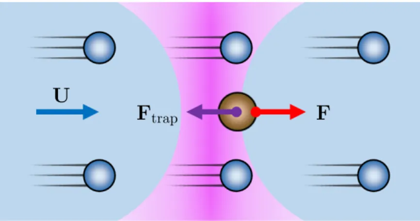
U F

F

Figure 2.5: Schema of experimental system studied by Wilson

is trapped by optical tweezers in a flowing colloidal suspension. Colloidal particles and a solvent flow at a constant velocity

exerted by the flowing suspension and the trapping force

caused by the optical tweezers. At steady states, the magnitude of

balances with that of

.

and cycloheptylbromide (CHB). They grafted poly-12-hydroxystearic acid (PHSA) on the PMMA particles and added tetrabutylammonium chloride to the solvent mixture so that the PMMA particles behaved as hard spheres. The refractive index of the solvent matched that of the PMMA particles (n = 1.49). The viscosity of the solvent was η

= 2.56 mPa · s measured by rheometer. Although Wilson et al. prepared two batches of the PMMA particles with radii b = 860 and 960 nm (measured by light scattering), there was no systematic difference between the results of these batches.

To measure mechanical properties of this colloidal suspension, they used probe particles made of melamine resin. These probe particles were coated with PHSA so that the interaction between the probe and colloidal particles was given by hard spheres. The radius of the probe particles was a = 1.04 µm measured by light scattering. The refractive index of the probe particles was n = 1.7 different from that of the colloidal particles and the solvent. Because of the mismatching of the refractive indices, the probe particles are trapped by optical tweezers in the colloidal suspension.

2.2.2 Method

Wilson et al. fixed the probe particles spatially by optical tweezers. The optical

tweezers trap microsize particles in the vicinity of a focus of a condensed laser

beam. If the trapped particles deviate from the focus, the particles are subject

to the restoring force directed to the focus. The magnitude of the restoring force

is determined from the deviation from the focus. Since the restoring force of the

optical tweezers is generated by refraction of a laser beam at the boundary between

trapped particles and a medium, the optical tweezers trap only the probe particles

with the refractive index different from that of the solvent.

η

(P e) /η

Pe

Figure 2.6: P´ eclet-number dependence of effective viscosity. This figure is from Wilson

[4].

(Pe) and Pe are defined by Eq. (2.33) and (2.34), respectively.

(Pe) is scaled by the solvent viscosity

= 2.56 mPa

s.

the sample stage at a constant velocity U relative to the laser trap (Fig 2.5). They measured positions of the trapped probe particles at steady states for various U and the volume fraction of the colloidal particles ϕ. In the experimental system, the trapped probe particles are subject to the drag force F exerted by the flowing colloidal suspension and the restoring force F

caused by the optical tweezers. At steady states, the magnitude of F balances with that of F

. Since the magnitude of F

is determined from the deviation from the focus of the condensed laser beam, F is obtained from the measurement of the positions of the probe particles.

2.2.3 Results

Wilson et al. determined the effective viscosity of the colloidal suspension η

(Pe) defined by

η

(Pe) = | F |

6πa | U | . (2.33)

Figure 2.6 represents the P´ eclet-number dependence of η

(Pe) for various values of the volume fraction ϕ. Assuming a = b, Wilson et al. defined Pe as

Pe = 2a

D

| U | , (2.34)

where D

is the diffusion coefficient of the probe particles in the solvent. Note

that Eq. (2.34) corresponds to Eq. (2.14) in the case of a = b. In Fig. 2.6, η

(Pe)

is scaled by η

. Theoretically, from Eq. (2.32), η

(Pe)/η

is expected to satisfy the relation

η

(Pe) η

= ϕ

2

( a + b b

)

D

D V (Pe) + 1, (2.35)

where D is the diffusion coefficient of the colloidal particles and V (Pe) is the normalized viscosity increment obtained by Squires and Brady (Fig. 2.4).

From Fig. 2.6, Wilson et al. stated that the results for ϕ = 0.3 and 0.45 showed the decrease in the effective viscosity at large values of Pe but the results for the other values of ϕ did not represent the decrease. They considered that the decrease in the effective viscosity might be related with the decrease in the normalized viscosity increment shown in Fig. 2.4. Similar results showing the decrease in the effective viscosity had been obtained by Meyer et al. [3] However, Wilson et al. also stated that the decrease in the effective viscosity might be caused by the correction of the measurement at the edge of a condensed laser beam.

I consider that it is difficult to regard the experimental results obtained by Wil- son et al. (Fig. 2.6) as the verification of the numerical result obtained by Squires and Brady (Fig. 2.4). First, the effective viscosity for ϕ = 0.3 and 0.45 decreases at Pe > 100 in Fig. 2.6, while the normalized viscosity increment in Fig. 2.4 de- creases at 1 ≤ Pe ≤ 100. Next, although Fig. 2.4 was obtained by assuming the dilute limit, values of ϕ in Fig. 2.6 (ϕ = 0.3 and 0.45) are so large that effects of interactions between the colloidal particles are not negligible. Furthermore, since error bars in Fig. 2.6 are large, it is difficult to see the Pe-dependence of the effec- tive viscosity clearly. I consider that the differences between the numerical results (Fig. 2.4) and the experimental results (Fig. 2.6) are caused by excessive simpli- fication in the study by Squires and Brady: neglect of the nonuniform solvent velocity field and interactions between colloidal particles.

2.3 Summary

Squires and Brady considered a simple model for active microrheology in a colloidal suspension (Fig. 2.1). They obtained the density field of colloidal particles around a probe particle by solving the Smoluchowski equation. In the limits of low Pe and high Pe, they obtained the approximate solutions to the Smoluchowski equation analytically. They also obtained the density field for arbitrary Pe by solving the Smoluchowski equation numerically. By using the obtained density field, they calculated the viscosity increment due to the colloidal particles [Eq. (2.29)]. The results (Fig. 2.4) show that the viscosity increment in the high-Pe limit is half of that in the low-Pe limit.

The results obtained by Squires and Brady have not been verified by experi-

mental studies of microrheology. Wilson et al. obtained the effective viscosity of a

hard-sphere colloidal suspension (Fig. 2.6) from the experiment of active microrhe-

ology using hard-sphere probe particles and the optical tweezers. Although some

addition, the Pe- and ϕ-dependence shown in Fig. 2.6 is different from that shown

in Fig. 2.4. I consider that the differences between these results are caused by

excessive simplification in the theoretical study: neglect of the nonuniform solvent

velocity field and interactions between colloidal particles. In my study, I examine

effects of the nonuniform solvent velocity field and interactions between particles

on probe particles in active microrheology.

Chapter 3

Two-fluid model

3.1 Introduction

In the theoretical study by Squires and Brady [7], the solvent velocity was assumed to be constant in the whole system (see Sect. 2.1). In fact, since motion of a solvent is disturbed by the probe and colloidal particles, the solvent velocity field should be nonuniform. However, the nonuniform solvent velocity field cannot be treated in the framework of the Smoluchowski equation used in their study. To consider the disturbance due to the particles, the solvent velocity field should be obtained simultaneously with the distribution of the particles. I consider that these difficulties can be resolved by use of the two-fluid model.

For the mixture of two types of fluids, the two-fluid model gives two equations of motion for the fluids [13–15]. This model has often been applied to polymer solutions and binary polymer blends by regarding an aggregation of polymers as a fluid. In my study, regarding colloidal particles and a solvent as two types of fluids, I apply the two-fluid model to a colloidal suspension (Chap. 5). Here, to treat interactions between the colloidal particles, I combine the density functional theory (DFT) with the two-fluid model (Chap. 5). In this chapter, referring to the study by Doi and Onuki [13], I derive the equations of motion of the two-fluid model as the preparation for my study.

3.2 Derivation of equations

3.2.1 Continuity equation and incompressibility condition

Here, I consider a complex fluid comprised of colloidal particles and a solvent, in which the velocity of the colloidal particles differs from that of the solvent velocity.

The velocity fields of the colloidal particles and the solvent are represented by

v

(r, t) and v

(r, t), respectively. The volume-fraction field of the colloidal particles

is represented by ϕ(r, t). I assume that the volume-fraction field of the solvent is

represented by 1 − ϕ(r, t). The continuity equation is derived from the conservation

law and expressed by

∂ϕ(r, t)

∂t = −∇ · (ϕ(r, t)v

(r, t)). (3.1) Additionally, the incompressibility condition is expressed by

0 = ∇ · [ϕ(r, t)v

(r, t) + (1 − ϕ(r, t))v

(r, t)]. (3.2)

3.2.2 Rayleigh’s variational method

To obtain the equations of motion for the colloidal particles and for the solvent, I employ the Rayleigh’s variational method [16, 17]. The equations of motion are derived from the condition that ϕ(r, t), v

(r, t), and v

(r, t) change with the lapse of time, minimizing the sum of the energy dissipation per unit time and the time derivative of the free energy of the complex fluid. I define the Rayleighian as

R = W

2 + ˙ F , (3.3)

where W is the energy dissipation per unit time and F is the free energy of the complex fluid. By use of the Rayleigh’s variational method, the equations of motion at steady states are obtained from the condition that the derivatives of R equal zero. The obtained equations do not include the terms of acceleration, which are derived from the Lagrangian formalism.

To obtain the equations of motion under the incompressibility condition [Eq. (3.2)], I add the term of the constraint condition to the Rayleighian defined by Eq. (3.3).

The modified Rayleighian including the constraint condition is given by R

= W

2 + ˙ F −

∫

p(r, t) ∇ · [ϕ(r, t)v

(r, t) + (1 − ϕ(r, t))v

(r, t)]dr, (3.4) where p(r, t) is the undetermined multiplier of the Lagrange multiplier method.

From the obtained equations, p(r, t) turns out to be the pressure field of the complex fluids. To determine the pressure field p(r, t) satisfying the incompress- ibility condition [Eq. (3.2)], I derive the equations of motion from the modified Rayleighian given by Eq. (3.4).

3.2.3 Energy dissipation

The energy dissipation W is the sum of the dissipation due to relative motion between the colloidal particles and the solvent W

and that due to the solvent viscosity W

. Here, W

is given by

W

=

∫

Γ(ϕ(r, t))(v

(r, t) − v

(r, t))

dr, (3.5)

where Γ(ϕ(r, t)) is the friction coefficient between the colloidal particles and the

solvent. In the Rayleigh’s variational method, W

is defined as the function

including only the second-order terms of v

(r, t). Additionally, to determine W

,

I make the following assumptions,

1. W

has the translational symmetry, so that it includes only the terms of the gradient of v

(r, t);

2. W

does not include the second- or higher-order differential terms of v

(r, t).

Under these assumptions, W

is given by W

= ∫ ∑

α,β

[ µ ∂v

∂x

∂v

∂x

+ (µ + λ) ∂v

∂x

∂v

∂x

]

dr, (3.6)

v

(r, t) = (v

, v

, v

), (3.7) where µ and λ are the shear viscosity and volume viscosity of the solvent, respec- tively, and α and β represent either of three components of the vector r.

3.2.4 Time derivative of free energy

The free energy F consists of the mixing free energy F

and the elastic free energy F

. The mixing free energy F

is generated by mixing the colloidal particles with the solvent. The elastic free energy F

is associated with the conformation of the constituting particles such as polymer chains. For simplicity, I assume that the conformation of the colloidal particles is in equilibrium so that F

is negligible. Additionally, I neglect the terms of ∇ ϕ(r, t) in F

, which arises from the inhomogeneity of ϕ(r, t). Here, F

depends on ϕ(r, t) only.

When F

is the functional of ϕ(r, t), F

is given by F

=

∫

f (ϕ(r, t))dr, (3.8)

where f (ϕ(r, t)) is the mixing free energy per unit volume with the volume-fraction field ϕ(r, t). From the continuity equation [Eq. (3.1)], the time derivative of F

is given by

F ˙

=

∫ ∂f (ϕ(r, t))

∂ϕ(r, t)

ϕ(r, t)dr ˙

= −

∫ ∂f (ϕ(r, t))

∂ϕ(r, t) ∇ · (ϕ(r, t)v

(r, t))dr. (3.9)

Since F

has been assumed to be negligible, the total free energy F corresponds

to F

. Therefore, the time derivative of F is given by Eq. (3.9).

3.2.5 Motion equations at steady states

Eventually, the modified Rayleighian is given by R

=

∫ { 1

2 Γ(ϕ(r, t))(v

(r, t) − v

(r, t))

+ 1

2

∑

α,β

[ µ ∂v

∂x

∂v

∂x

+ (µ + λ) ∂v

∂x

∂v

∂x

]

− ∂f (ϕ(r, t))

∂ϕ(r, t) ∇ · (ϕ(r, t)v

(r, t))

− p(r, t) ∇ · [ϕ(r, t)v

(r, t) + (1 − ϕ(r, t))v

(r, t)]

}

dr. (3.10)

The equation of motion for the colloidal particles at steady states is obtained from the condition that the functional derivative of R

by v

(r, t) equals zero. The obtained equation for the colloidal particles is given by

0 = Γ(ϕ(r, t))(v

(r, t) − v

(r, t)) + ϕ(r, t) ∇ ∂f (ϕ(r, t))

∂ϕ(r, t)

+ ϕ(r, t) ∇ p(r, t). (3.11)

In the same way, the equation of motion for the solvent is obtained from the functional derivative of R

by v

(r, t). The obtained equation for the solvent is given by

0 = Γ(ϕ(r, t))(v

(r, t) − v

(r, t)) + (1 − ϕ(r, t)) ∇ p(r, t)

− µ ∇

v

(r, t) − (µ + λ) ∇ ( ∇ · v

(r, t)). (3.12)

3.2.6 Approximate incompressibility condition

In addition to the incompressibility condition given by Eq. (3.2), I consider the approximate incompressibility condition defined by

0 = ∇ · v

(r, t). (3.13)

This is the standard incompressibility condition for a simple fluid composed of a solvent. The approximate incompressibility condition is accurate in the dilute limit because the incompressibility of the colloidal particles is neglected in Eq. (3.13).

Under this incompressibility condition, the energy dissipation due to the solvent viscosity W

is given by

W

= µ

∫

dr ∑

α,β

∂v

∂x

∂v

∂x

. (3.14)

From Eqs. (3.13) and (3.14), the modified Rayleighian is given by R

=

∫ { 1

2 Γ(ϕ(r, t))(v

(r, t) − v

(r, t))

+ 1 2

∑

α,β

µ ∂v

∂x

∂v

∂x

− ∂f (ϕ(r, t))

∂ϕ(r, t) ∇ · (ϕ(r, t)v

(r, t)) − p(r, t) ∇ · v

(r, t) }

dr. (3.15)

From the condition that the functional derivative of R

by v

(r, t) equals zero, the equation of motion for the colloidal particles at steady states is obtained,

0 = Γ(ϕ(r, t))(v

(r, t) − v

(r, t)) + ϕ(r, t) ∇ ∂f (ϕ(r, t))

∂ϕ(r, t) . (3.16) In the same way, the equation of motion for the solvent is obtained from the functional derivative of R

by v

(r, t),

0 = Γ(ϕ(r, t))(v

(r, t) − v

(r, t)) + ∇ p(r, t) − µ ∇

v

(r, t). (3.17)

These equations are simpler than Eqs. (3.11) and (3.12). However, note that

Eqs. (3.16) and (3.17) are accurate only in the dilute limit.

Chapter 4

Application of time-dependent density functional theory to

numerical study of microrheology

4.1 Introduction

Squires and Brady considered a simple model for active microrheology in a colloidal suspension and obtained the force exerted by colloidal particles on a probe particle (see Sect. 2.1). In their study, they assumed the dilute limit and neglected effects of interactions between colloidal particles. In this chapter, I examine effects of interactions between colloidal particles on the force acting on a probe particle via numerical calculations. Here, I consider a simple model for active microrheology in a colloidal suspension similar to that studied by Squires and Brady. To examine effects of interactions between colloidal particles, I employ the time-dependent density functional theory (TDDFT).

The TDDFT is a powerful tool for studying effects of interactions between particles [18–38]. In particular, this theory has been successful in describing the dynamics of simple liquids [18–33]. For instance, the application of the TDDFT has allowed one to examine effects of interactions between solvent particles on the dynamics of them around a solute [18–26]. The TDDFT has also been applied to systems of large particles constituting soft matter because the application of the TDDFT is not restricted by particle size [34–38]. Applying the TDDFT to a system of active microrheology in a colloidal suspension, I examine effects of interactions between colloidal particles via numerical calculations [11, 12].

4.2 Model and method

4.2.1 Model system

A probe particle is fixed at the origin in a colloidal suspension flowing at a constant

velocity U (Fig. 4.1). Here, I focus on the force F exerted by the colloidal particles

on the probe particle. I assume that the probe and colloidal particles are hard

U

F

Figure 4.1: Model system for active microrheology in colloidal suspension. A probe particle is fixed spatially in a colloidal suspension. The colloidal suspension flows at a constant velocity

exerted by the colloidal particles. The probe and colloidal particles are hard spheres with radii

and

spheres with radii a and b, respectively. The colloidal particles interact with each other as well as with the probe particle. To examine effects of the hard-sphere interactions between the colloidal particles on F, I calculate the density field of the colloidal particles at steady states.

This system (Fig. 4.1) is similar to the system studied by Squires and Brady (Fig. 2.1) [7]. In the same way as their study, I assume that the solvent velocity is constant in the whole system. However, unlike their study, the colloidal particles interact with each other in the system shown in Fig. 4.1. To study effects of interactions between the colloidal particles, I employ the time-dependent density functional theory (TDDFT).

4.2.2 Time-dependent density functional theory

Applying the TDDFT to the system shown in Fig. 4.1, I calculate the temporal development of the density field of the colloidal particles ρ(r) by the basic equation [18, 34, 35, 39],

∂ρ(r, t)

∂t + U · ∇ ρ(r, t) = D ∇ · (

ρ(r, t) ∇ δβF [ρ(r, t)]

δρ(r, t) )

. (4.1)

Here, D is the diffusion coefficient of the colloidal particles, β = 1/k

T , and

F [ρ(r, t)] is the free-energy functional of ρ(r, t). In Eq. (4.1), the second term on

the left-hand side is the advective term arising from the flux of the colloidal suspen-

sion. Because of the advective term with constant U, ρ(r, t) is in a nonequilibrium

steady state even in the t → ∞ limit. The boundary condition for Eq. (4.1) is

that ρ(r, t) equals the homogeneous density ρ

far from the probe particle.

the Legendre transformation; F [ρ(r, t)] is obtained from the Legendre transforma- tion of the thermodynamic potential which is defined by the virtual external field that the intensive variable paired with ρ(r, t). The derivation of the equation of F [ρ(r, t)] is explained in detail in Append. B. When the density field ρ(r, t) is close to the homogeneous density ρ

, F [ρ(r, t)] is given by [18, 21, 39]

βF [ρ(r, t)] = βF

[ρ(r, t)] − βΨ[ρ

]

− ∑

n=1

1 n!

∫

c

(r

, · · · , r

)∆ρ(r

, t) · · · ∆ρ(r

, t)dr

· · · dr

, (4.2) where

Ψ[ρ(r, t)] = F

[ρ(r, t)] − F [ρ(r, t)], (4.3)

∆ρ(r, t) = ρ(r, t) − ρ

. (4.4)

The n-particle direct correlation function c

(r

, · · · , r

) is defined in the homoge- neous system which is in the absence of the probe particle,

c

(r

, · · · , r

) = βδ

Ψ[ρ(r, t)]

δρ(r

, t) · · · δρ(r

, t)

ρ(r,t)=ρ0

, (4.5)

and F

[ρ(r, t)] is the free-energy functional for ideal gas, βF

[ρ(r, t)] =

∫

ρ(r, t)[ lnρ(r, t) + βV (r) + lnΛ

− 1 ]dr. (4.6) Here, V(r) denotes the interaction between the probe and colloidal particles and Λ is the thermal de Broglie wave length given by

Λ =

( h

2πmk

T

)

, (4.7)

where h is the Planck’s constant and m is the mass of a colloidal particle.

To obtain a computable expression of Eq. (4.2), I neglect the three- and more- particle direct correlation functions. Hence, I obtain the free-energy functional F [ρ(r, t)],

βF [ρ(r, t)] = βF

[ρ(r, t)] − βΨ[ρ

] − c

∫

∆ρ(r, t)dr

− 1 2

∫

c

(r

− r

)∆ρ(r

, t)∆ρ(r

, t)dr

dr

. (4.8)

The neglect of the three- and more-particle direct correlation corresponds to the

hypernetted-chain (HNC) approximation [40]. In the interest of consistency, the

HNC approximation should be employed in the calculation of c

(r). By substitut- ing Eq. (4.8) into Eq. (4.1), I obtain

∂ρ(r, t)

∂t + U · ∇ ρ(r, t) = D ∇ · [

∇ ρ(r, t) + βρ(r, t) ∇ V (r)

− ρ(r, t) ∇

∫

c

(r − r

)∆ρ(r

, t)dr

]

, (4.9)

where the convolution-integral term of c

(r − r

) is related to the interactions between the colloidal particles.

In order to examine effects of the interactions between the colloidal particles, I also calculate the density field of noninteracting colloidal particles. The non- interacting colloidal particles do not interact with each other, but they interact with the probe particle through the potential V (r). Thus, the noninteracting col- loidal particles are the same as the colloidal particles in the studied by Squires and Brady [7]. By removing the term of c

(r) from Eq. (4.9), I obtain the equation of the TDDFT for the noninteracting colloidal particles [7, 9, 10],

∂ρ

(r, t)

∂t + U · ∇ ρ

(r, t) = D ∇ · [ ∇ ρ

(r, t) + βρ

(r, t) ∇ V (r)]. (4.10) I calculate the density field at steady states ρ

(r, ∞ ) by solving Eq. (4.10), and determine the effects of the interactions from the difference between its value and ρ(r, ∞ ).

4.2.3 Application to system of hard-sphere particles

Applying the TDDFT to the system comprised of hard-sphere particles (Fig. 4.1), I calculate density fields of the colloidal particles at steady states. In this system, I define V (r), the interaction between the probe and colloidal particles, as

V (r) =

{ ∞ , at | r | < a + b,

0, at | r | ≥ a + b, (4.11)

where a and b are the radii of the probe and colloidal particles, respectively. Here, the origin of the vector r is placed at the center of the probe particle. The in- teraction between the colloidal particles is also given by the hard sphere with the diameter 2b. By substituting Eq. (4.11) into Eqs. (4.9) and (4.10), I obtain the equations of the TDDFT for | r | ≥ a + b,

∂ρ(r, t)

∂t = D ∇

ρ(r, t) − U · ∇ ρ(r, t)

− D ∇ · [

ρ(r, t) ∇

∫

c

(r − r

)∆ρ(r

, t)dr

]

, (4.12)