Hyperspectral remote sensing of soil salinity in Minqin oasis, China

(1)

I

Hyperspectral remote sensing of soil salinity in Minqin oasis, China

(

)

Qian Tana

The United Graduate School of Agricultural Sciences Tottori University, Japan

2018

(2)

I

Hyperspectral remote sensing of soil salinity in Minqin oasis, China

(

)

A dissertation submitted to

The United Graduate School of Agricultural Sciences, Tottori University In partial Fulfillment of the Requirements for the Degree of Doctor of

Philosophy

Qian Tana

The United Graduate School of Agricultural Sciences Tottori University, Japan

2018

(3)

I

ACKNOWLEGEMENTS

First of all, I would like to express my deepest gratitude to my principal supervisor Prof.

Tsunekawa from Arid Land Research Center (ALRC) of Tottori University for precious academic advising for my research, also enthusiastic help, and strong support for all the time.

Great appreciation also given to my co-supervisor Masunaga sensei from Shimane University as well as Prof. Peng who gave me great numbers of valuable suggestions on research design, result analysis, field survey and paper writing. Researching about soil was an impossible mission for a student like me had never learned about soil science before. Because of their encouragement and supports, I can finally fulfil my PhD dream successfully. I also appreciate Professor Kitamura Yoshinobu. He sacrificed a lot of time on helping me figure out my questions about soils and carefully helped me checking my manuscript. I enjoyed the wonderful researches experience with all the professors, which is invaluable wealth for my whole life. Great appreciation also given to Prof. Fujimaki, he taught me about soil knowledge and how to measure the Electivity Conductivity of soil and also borrowed me some equipment.

I would like to thank water resources bureau in Minqin County for sharing important background information and data about water resources in Minqin oasis; the Mr. Wang who is a local farmer and helped me and be the driver during my field survey in Minqin; the local farmers who I have interviewed during field survey in Minqin County for their cooperation.

I would like to thank Professor Xue Xian, Professor Wang Ninglian, Dr. Huang Cuihua, Dr. Liao Jie, Dr. Luo Jun and Dr. Dong Siyang from Northwest Institute of Eco-Environment and Resources, CAS, for providing them with the equipment and the assistance during field survey in China; Professor Wei Huaidong, Professor Ding Feng and Professor Zhou Liping, from Gansu Desertification and Aeolian Sand Disaster Combating Institute for providing them with the equipment and the assistance in the measurement; Professor Kitamura Yoshinobu and Professor Fujimaki Haruyuki from Tottori University for the useful advices and equipment.

Special thanks are given to the members of Plant Production lab and staff of Arid Land Research Center (ALRC) for their help and cooperation in my life. They are Tomemori san,

(4)

II

Sakei san, Miyata san, Kobayashi Nobuyuki, Derege, Shunsuke Imai, Du Wuchen, Gou Xiaowei, Chen Xiang, Dagnenet Sultan, Kindye Ebabu, Zerihun Negussie, Fanthun Aklog, Misganaw Teshager, Mesenbet Yibltal, Mulat Liyew, Fekerimaram Asaregew, Shigdaf Mekuriew, Gashaw Tena, Birhanu Kebebe, Getu Abebe. I had a good time with all the lab- members when pleasant exchanging our cultural difference and sharing stories.

I indebted thank to my parents and my grandma who have always supported and always encouraged me. I feel guilty that they are getting old without their beloved daughter and

optimistically face the difficulties in my study and life. I am, so grateful to be surrounded by people I love with all my heart and so thankful for my family and their never ending love and support. I will keep doing my best in my life and bring them more happiness.

I would like to thank to all my friends, who helped and encourage me and spending wonderful fun time with me during my Ph.D.

ssion, frustration and self-assurance issues over a long time of my PhD period. However, at the same time I felt challenges, excitement and fulfillment that doing research have brought me with. I think this toughness and failure over PhD life, she or he perhaps eventually will be physically and mentally stronger for anything might happen in their life. Thanks to myself for not giving up.

(5)

LIST OF FIGURES

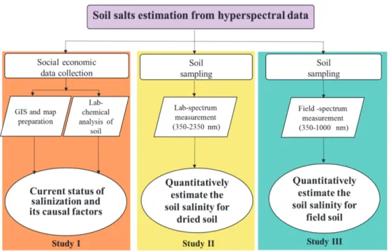
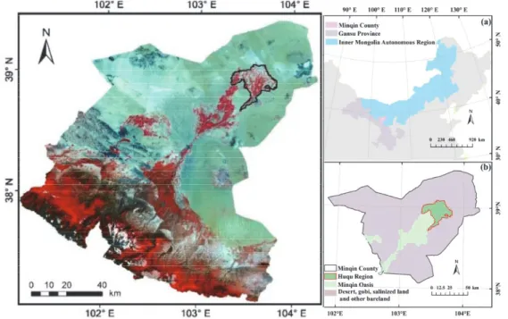
Fig. 1 The integrated methodology of the thesis ...9 Fig. 2 (a) The location of the study area (the Huqu region) within China, (b) Locations of the 94 soil samples analyzed in the present study. ...10 Fig. 3 (a) the total number of well in Minqin County; (b) the ground water table level of Minqin County (c) the ground water table level of Huqu region; (d) the total dissolved salt of ground water of Minqin County. ...13 Fig. 4 The summary of salinization process in Minqin oasis. ...15 Fig. 5 Locations of the 94 soil samples analyzed in the present study...18 Fig. 6 Histograms of EC1:5 values for samples from (a) cropland (n = 21) and (b) all other land types (n = 73), and their associated descriptive statistics ...23 Fig. 7 Map of the distribution of EC1:5 values for the 94 soil samples...24 Fig. 8 Topographic map of the study area showing locations of 64 soil sampling sites. ...33 Fig. 9 Concentrations of Na⁺, K⁺, Ca²⁺, Mg²⁺, Cl , SO42 and HCO3 ions in samples for each of the five ranges of soil salinity defined in section 2.2. The percentage concentration for each ion was calculated as its concentration divided by the total cation and anion concentration for that salinity range. ...38 Fig. 10 Reflectance spectra: (a) original measured spectra of all 64 soil samples, (b) averaged spectra of samples in five salinity ranges, (c) CR-reflectance spectra of samples in five salinity ranges, (d) enlargement of panel for range of 1344 1619 nm, (e) enlargement of panel for range of 2241-2387 nm, (f) enlargement of panel for range of 2422 2488 nm. .40 Fig. 11 Heatmap of correlation coefficients (r) for correlations of wavebands of measured

salinities with all candidate NDSI waveband pairs ...41 Fig. 12 (a) Measured soluble salt content (SSC) versus normalized difference spectral index (NDSI) and (b) scatter plot of measured SSC versus SSC estimated from Eq. 5 ...42 Fig. 13 Correlation coefficients (r) obtained for correlations of measured concentrations in our samples of seven ions and organic carbon content (OCC) with CR-reflectance at 2382 and 1358 nm, and with the NDSI we developed in this study. Correlations were significant at the 0.01 probability level except for correlations of CR-reflectance at 2392 nm with HCO3, CR-reflectance at 1358 nm with Ca²⁺, and NDSI with HCO3 , which were significant at the 0.05 probability level. ...43 Fig. 14 Topographic map of the study area showing locations of 58 soil sampling sites. ...46 Fig. 15 Concentrations of Na⁺, K⁺, Ca²⁺, Mg²⁺, Cl , SO42 and HCO3 ions in samples for each of the five ranges of soil salinity defined in section 2.2. The percentage concentration for each ion was calculated as its concentration divided by the total cation and anion concentration for that salinity range. ...48 Fig. 16 (a) The spectrum of original reflectance for 58 soil samples (b) the correlation coefficient for original reflectance and SSC for 58 soil samples. ...49 Fig. 17 (a) Heatmap of correlation coefficients (r) for measured salinities and all waveband pairs candidates from original reflectance data in difference form (b) heatmap of correlation

(8)

VI

coefficients (r) for measured salinities and all waveband pairs candidates from original reflectance data in NDSI form ...50 Fig. 18 (a) the spectrum of first derivate of reflectance for 58 soil samples (b) the correlation coefficient for first derivate values of spectrum and SSC for 58 soil samples. ...51 Fig. 19 (a) Heatmap of correlation coefficients (r) for measured salinities and all waveband

correlation coefficients (r) for measured salinities and all waveband pairs from first derivate reflectance data candidates in NDSI form ...53 Fig. 20 (a) Scatter plot graph for measured salinities and difference index of first derivate

reflectance data (b) scatter plot graph for measured salinities and NDSI of first derivate reflectance data. ...54 Fig. 21 (a) The spectrum of continuum removed reflectance for 58 soil samples (b) the

correlation coefficient for continuum removed reflectance and SSC for 58 soil samples. .55 Fig. 22 (a) Heatmap of correlation coefficients (r) for measured salinities and all candidate

waveband pairs in difference based on difference index, (b) heatmap of correlation coefficients (r) for measured salinities and all candidate waveband pairs in difference based on NDSI ...56 Fig. 23 (a) Measured soluble salt content (SSC) versus normalized difference spectral index (NDSI) and (b) scatter plot of measured SSC versus SSC estimated from Eq. 5. ...57 Fig. 24 (a) Soil moisture content (SMC) versus Residue of predicted SSC and measured SSC and (b) Soil moisture content (SMC) versus normalized difference spectral index (NDSI).

...58 Fig. 25 (a) the calibration of model1, (b) the calibration of model 2, (c) the calibration of model 3, (d) the calibration of model 4, (e) the calibration of model 5. ...62 Fig. 26 (a) Measured soluble salt content (SSC) versus normalized difference spectral index (NDSI) formed by band 489 and 1358 (b) Measured soluble salt content (SSC) versus normalized difference spectral index (NDSI) formed by band 517 and 2382. ...63 Fig. 27 Measured soluble salt content (SSC) versus predicted soluble salt content (SSC)...64

(9)

LIST OF TABLES

Table 1 World distribution of salt-affected soils ...6

Table 2 Monthly mean temperature and mean precipitation of Minqin County ... 11

Table 3 Definitions of the affecting factors for the reference series (soil EC1:5) ... 22

Table 4 Descriptive statistics for the soil parameters, by land use and cover class (LUCC)a ... 26

and the resulting ranking for each affecting factor ... 27

ing ranking for the two main land use and cover types ... 28

Table 7 Descriptive statistics of chemical properties of 64 soil samples ... 37

Table 8 Correlation matrix of relationships between variables ... 37

Table 9 Descriptive statistics of chemical properties of 59 soil samples ... 48

Table 10 Correlation matrix of relationships between variables ... 48

Table 11 Total variance explained ... 59

Table 12 The correlation between soil properties and PCA factors ... 59

Table 13 ANOVA ... 60

Table 14 The coefficients of models^a ... 61

(10)

VIII

ACRONYMS AND ABBREVIATIONS

ASD Analytical spectral devices

ASTER GDEM Aster global digital elevation model CV Coefficient of variation

CTI Compound topographic index

CR Continuum removal

DEM Digital elevation model

EC Electrical conductivity

ECe EC of saturated soil paste extract, dS/m EC1:5 EC of 1:5 soil and water ratio, dS/m GIS Geographical information systems GRA Grey relational analysis

HRS Hyperspectral remote sensing

NDSI Normalized difference spectral index

NIR Near infrared

OCC Organic carbon content OMC Organic matter content PCA Principal component analysis

PCs Principal components

SAR Sodium adsorption ratio

SD Standard deviation

SI Salinity index

SWIR Shortwave infrared

NDSI Soil salt index

SMC Soil moisture content SSC

TDS

Soluble salt content Total dissolved salt

VIS Visible infrared

VNIR Visible-near infrared reflectance MASL Meters above mean sea level

(11)

Chapter 1

General Introduction

(12)

2

Chapter 1 General Introduction

1.1 Background

Soil salinization is the most common type of land degradation encountered in natural resource management in many parts of the world and has received much attention from farmers, politicians and researchers (Wild, 2003; Rengasamy, 2006;

Farifteh et al., 2006; Sheng et al., 2010; Wang et al., 2018). It possesses the potential to cause extensive environmental degradation, health issues and economic welfare. Its occurrence is generally characterized by the appearance of bare salty patches, sparse vegetation cover density, and the appearance of salt tolerant plants and/or the salinization of water resources (Greiner, 1998; Walker et al., 1999). Salinization refers to the process of the accumulation of water-soluble salts in the soil to a level that impacts on agricultural production and environmental health. It commonly occurs as a result of irrigated agricultural practices or long-term changes in water flow in the landscape or changed water management (Pitman and Läuchl, 2002).

Salinization can be caused by natural and/or human activities. In semi-arid and arid land, salinization occurs in one of three situations: salt input increases, freshwater input decreases, or freshwater extraction increases. Under some conditions, all of these processes occur naturally, and in this case are known collectively as primary salinization. For instance, water soluble salts are carried by inland rivers flowing from mountains in upper stream to downstream and form the terminal water bodies. Under drought conditions, salinity of inland waters will increase when decreased precipitation and evaporation results in decreased freshwater input to the soil. In the downstream, without natural outlets, the water bodies fed by river runoff will gradually decreasing in volume and increasing in salinity through evaporation. In this case, it is known as natural or primary salinization process.

Human activity interference leads to the three salinization mechanisms increase rapidly, particularly in dryland and in agricultural systems. Salinization affected by anthropogenic factors is also known as secondary salinization. Human activities that disrupt the hydrologic balance of the soil between water applied (irrigation or rainfall)

(13)

and water used by crops (transpiration). In many irrigated areas, the groundwater table has raised due to excessive irrigation and the insufficient drainage as well as the removal of indigenous vegetation to make room for cultivated lands and pastures (the decreased demand for groundwater causes the water table to rise). The resource of excessive irrigation are generally comes from the extraction of freshwater from inland bodies (surface runoff and/or groundwater) which reducing the lake area and further concentrating salts (Nurmemet et al. 2015). The accumulation of soluble salts in the root zone greatly affects plant growth, resulting in lower crop production and adversely affecting the soil fertility. As one of the primary inhibitors of agricultural production and ecosystem, salinization might ultimately lead to environmental disaster and food crises in arid lands (Munns, 2002; Barrett-Lennard, 2003).

Soil salinity is defined as the salt content in the soil. Salinity in water can be measured in two ways: total dissolved solids (TDS) and electricity conductivity (EC) of a saline solution. The metric unit for conductivity is the deci-Siemens per meter (dS/m) (Paul and Rashid, 2016). The excess salts in the soil solution are comprised largely of the chloride and sulfate anions and sodium, magnesium, and calcium cations (Qingfeng Lv et al., 2018). It results in poor plant growth and low soil microbial activity due to osmotic stress and toxic ions (Yan et al., 2015). Threshold value of soil salinity classes deleterious effects occur can vary from one environment to another depending on several factors including plant type, soil-water regime and climatic condition (Maas et al. 1986). According to FAO 1985, the soil is said to be non-saline if the saturation extract water contains less than 3 grams of salt per litre or 4.5 mmhos/cm, and the soil is said to be highly saline if the salt concentration of the saturation extract contains more than 12 g/L. However, based on Albert (Canada) Agriculture and Forestry, non-saline soils are defined as EC of salt solution <2 dS/m, and strongly saline soils are the soils have EC >8 dS/m, very strongly saline soils have EC >16 dS/m. Therefore, site-specific classification is needed (Paul and Rashid, 2016).

Salinization has become a serious threat to the agriculture and the livelihood of residents in the arid north western China. Their agriculture is heavily rely on the river

(14)

4

problems that are strongly affecting agricultural development and sustainability. The low precipitation is coupled with intensive evaporation and ineffective irrigation drainage systems have resulted in secondary salinization (Ma et al., 2005; Wang et al., 2008).These problems are especially severe in oasis ecosystems, where the water scarcity and soil salinization have caused an unrepairable loss of productive land within the past few decades and have threatened the sustainability of agriculture and ecosystem stability. ). Among the numerous inland river basins in the Northwest China, the lower reach of the Shiyang River Basin is well-known for its serious water shortage and the deteriorated eco-environment, which have impeded the social and economic development (Wang, 2009). Minqin oasis, in the lower reaches of the Shiyang River (an inland river rising in the Qilian Mountains), suffers a great shortage of fresh water for agriculture because of the low rainfall and massive demand for water created by increased agricultural activity and rapid population growth. Groundwater has been over-exploited to fill the gap between surface freshwater supply and demand (Bondes and Li, 2013; Wei, 2016). Groundwater extraction provides short-term relief from the scarcity of water for agricultural and domestic use, but excessive extraction lowers the water table and increases salt concentrations in groundwater (Chen et al., 2016). Long- term agricultural use of saline water has led to a rapid increase of secondary salinization at Minqin oasis (Chen et al., 2016; Qian et al., 2017). For example, the total area of saline land within Minqin oasis increased by 541.35 km² from 1991 to 2009 (Xiao et al., 2007; Zhang et al., 2014). Moreover, the persistent water scarcity and adverse effects of secondary salinization on crop yields led to the abandonment in 2003 of about 780 ha of cropland (equal to 81% of area under cultivation) at two villages at Minqin oasis (Ma et al., 2007).

(15)

1.2 Literary review

1.2.1 Salinization in the world

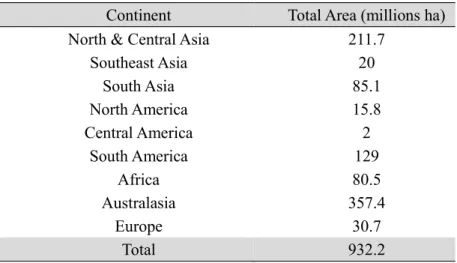
Soil salinization is a universal problem, especially in much of the waterfront, arid and semi-arid lands of more than 100 countries and regions over different continents (Table 1). Irrigation-induced land salinization has put serious risks to the sustainability of irrigated agriculture (Singh et al., 2012). Arable land affected by salts accounts for 23% of global arable land (Scudiero et al., 2016). About 17% of the global cropland is under irrigation, but irrigated agriculture accounts for over 30% of the total production (Hillel, 2000). Therefore, secondary salinization is of major concern for world food production. An estimations of the proportion of secondary salinization soils to its irrigated for several countries are 8.7 % for Australia, 15% or China, 16.6 % for India, 23 % for USA, 33 % for Egypt, 33.7 % for Argentina,

Paul and Rashid, 2016).

has enlarged considerably during the last few decades with a spreading rate of 2 million ha per year due to the speedy expansion of irrigation (Singh, 2010; Singh, 2011).

In Australia, 16% of the cropping area (7.6×10⁶ km) is likely to be affected by water table-induced salinity, 67% of the area

Aus$1330 million per annum. In recent years, many farmers have abandoned their rice fields due to the adverse impact of soil salinization (Rengasamy, 2006).

In Pakistan, an estimates show that 25% and 40% of the irrigated lands in the Punjab and Sindh are salt-affected respectively, which impacts on the livelihoods of about 10 20 million people and ecosystem (Barrett-Lennard and Hollington, 2006).

Soil salinization restricts agricultural development, especially when sustainable agricultural development and environmental quality improvement strategies are being considered. In Bangladesh, due to increasing degree of salinity and expansion of affected areas normal agricultural land use practices become more restricted (Karim et al., 1990). Large area of the coastal and off-shore lands of arable lands are affected by varying degrees of salinity (Asib, 2011). Though salinity mapping, a research showed

(16)

6

that, saline and highly saline areas covered about 3336.67 hectares and 2941.94 hectares respectively which are 41.46% and 36.69% land of total study area of their study sites (Mohamed et al., 2012).

Table 1 World distribution of salt-affected soils

Continent Total Area (millions ha) North & Central Asia 211.7

Southeast Asia 20

South Asia 85.1

North America 15.8

Central America 2

South America 129

Africa 80.5 Australasia 357.4

Europe 30.7

Total 932.2

Reproduced from Sumner Szabolcs, 1989.

1.2.2 Method and techniques of retrieving soil salinity

Even though the effects of spatiotemporal variations of natural conditions (e.g., availability of irrigation water) and the temporal changes of agricultural practices have made it difficult to monitor and manage the salinization, the accurate estimations of the areal extent of salt affected soil and prediction of areas has potential to become saline are essential for policy makers, planners and farmers to allow effective management of irrigated land, control of salinization and reversal of current trends of soil and water degradation. Thus, it is crucially important to monitor soil salinity and assess its severity to prevent further degradation of agricultural land (Weng et al., 2010).

Conventionally, soil salinity has been measured by collecting in situ soil samples and analysing those samples in the laboratory to determine their solute concentrations or electrical conductivity (EC). EC can be measured in saturated paste extracts (ECe) or by using extracts with different soil-to-water ratios (Shainberg and Levy, 2005).

Because the conventional methods of monitoring salinity by using ground-based geophysical techniques are time-consuming and costly (Dehaan and Taylor, 2003) soils have high spatial variability, many researchers have attempted to develop more cost-

(17)

effective approaches by utilizing remote sensing techniques to monitor the salt-affected soils and predict the potential salinization (Metternicht and Zinck 2003; Farifteh et al.

2007; Mulder et al. 2011).

Remote sensing uses the electromagnetic energy reflected from targets to obtain spectral information about the land surface in details. Spectral information enables the identification of object based on its spectral features such as reflection, absorption, and/or emit of electromagnetic energy at specific wavelengths. Compared with limit band numbers and resolutions of multispectral remote sensing techniques, hyperspectral remote sensing techniques have hundreds of bands, long wavelength, and high spectral resolution. It can capture subtle differences in soil properties and provide quick indirect assessments of soil characteristics such as salinity, organic content and moisture content (Ben-Dor and Banin, 1995; Farifteh et al., 2006; Gomez et al., 2008;

Haubrock et al., 2008; Zornoza et al., 2008; Ben-Dor et al., 2009; Goetz, 2009). Because the reflectance spectra of soils can provide quantitative information about the particular salt minerals in soils, the development of methods that use hyperspectral data to estimate soil salinity has been the objective of many studies during the past two decades (Farifteh et al., 2006; Gomez et al., 2008; Haubrock et al., 2008; Lu et al., 2013).

Hyperspectral visible and near-infrared reflectance spectroscopy displays promise as a result of its performance, accuracy and cost effectiveness in the determination of most soil properties in laboratories (Shepherd and Walsh, 2002).

Soil spectral reflectance is affected by many soil properties such as parent material, types of soil texture, soil moisture, salt content, colour, surface roughness, organic matter content, particle size, iron oxide content and texture (Farifteh, 2007), vegetation cover, vegetation types and vegetation growth conditions (Weng and Gong, 2006).

The dynamic processes of salinization also affect the spectral, spatial and temporal behaviour of the soil salts. The spectral reflectance of features vary with the change of those affecting factors, including salt crusts and efflorescence besides variations in surface texture and structure. Schmid et al. confirmed the fact that saline soil reflectance results from spectral properties such as the presence of salt crust, soil colour and

(18)

8

found that crusted saline soil reflects strongly in the visible and near-infrared (NIR) bands. Spectral reflectance of soil salt features can be promising surface indicators of soil salinity and spectral-based models can be generated to predict or mapping salinization. Fernandez et al. used the correlation between surface colours, EC and the sodium adsorption ratio (SAR) to predict soil salinity. This is based on the fact that the capabilities of different salt minerals to reflect and absorb light at particular band regions of the electromagnetic spectrum (Mougenot et al., 1993; Metternicht and Zinck, 2003).

Single or multiple wavebands that are sensitive to soil salinity in those areas of the spectrum can be mathematically combined (e.g., in ratio form, normalized ratio form, normalized difference form) into indices that can be used for modelling, detecting and mapping of soil salinity as well as other unidentified parameters (Douaoui et al., 2006).

A number of researchers have developed different salinity indices to detect and map soil salinity such as Normalized Difference Salinity Index and Salinity Index (Allbed and Kumar, 2013). Empirical models based on those indices can be used to predict salt concentrations in soil (Farifteh et al., 2007).

However, the complexity of soil properties makes identification of salt minerals in soil difficult and limit the monitoring and assessment of the salinization (Csillag et al.,1993), compounded by the fact that halite has an essentially featureless spectrum in the optical wavelength (Crowley, 1991). The spectral features that can vary according to the dominant salt present (e.g., NaCl or CaSO4), the sampling season and the area sampled (Metternicht and Zinck, 1997; Farifteh et al., 2007), which makes it difficult to define a general model that is applicable across large areas (Chang et al., 2001; Ben- Dor et al., 2002; Weng et al., 2010; Fan et al., 2015). The above shortcomings indicate that detecting and mapping soil salinity in arid and semi-arid regions using remote sensing is remain challenging.

1.4 Aims of the research

This research aims at quantifying soil salinity in soils on the basis of the use of soil reflectance and field survey, and investigate the potential of field and lab-derived

(19)

spectra for estimation salinity through comparison.

The specific objectives of this research are:

(a) To establish spatial distribution of soil salinity and analyzing its casual factors and to evaluate the effect of land use practices on the regional scale salinization;

(b) To quantitatively estimate soil salinity by modeling from lab-measured spectral reflectance data;

(c) To quantitatively estimate soil salinity by modeling from field-measured spectral reflectance data.

1.5 Structure of thesis

The thesis is organized into 5 chapters. After this introductory chapter, Chapter 2 (Study 1) detects the spatial variation of soil salinity and its causal factors in Minqin oasis. Chapter 3 (Study 2) derives the salt content in salinized soil from lab- hyperspectral reflectance data. Chapter 4 (Study 3) derives the salt content in salinized soil from field-hyperspectral reflectance data. The last chapter, Chapter 5, provides summarize of previous chapters. It includes conclusions, limitations of the study, and future research.

Fig. 1 The integrated methodology of the thesis

(20)

10

1.6 Study area description

1.6.1 Location

Minqin oasis is administratively named Minqin County of Gansu Province, northwestern China. The total area of Minqin County is about 1.6*10⁴ km²and lies

between . The Huqu region

is located on the downstream alluvial plain of the Shiyang River basin, in the northern part of the Minqin oasis. The terrain is relatively flat, with an elevation that ranges from 1254 to 1376 masl. It covers an area of 1430 km²

2-a). The region is surrounded by the Badan Jaran Desert to the west and north, and by the Tengger Desert to the east.

Fig. 2 (a) The location of the study area (the Huqu region) within China, (b) Locations of the 94 soil samples analyzed in the present study.

1.6.2 Climate

The region belongs to desert-oasis ecotone and has a temperate continental arid climate with more winds in winter and spring. The mean annual temperature is 7.8 °C with monthly means range from -8.6°C in January to 21.8°C in August. The frost-free period is 189 days roughly during April to October. The growing season for vegetation including crops are from March to October. The total annual precipitation averages 110

(21)

mm occurring in the summer months, but the potential evaporation ranges between 2000 and 2600 mm. The mean annual wind speed is 2.8 m/s, but the highest wind speed can reach 23 m/s, and winds strong enough to entrain sand occur 139 days per year on average (Local chronicles office of Minqin Count, 2014).

Table 2 Monthly mean temperature and mean precipitation of Minqin County

Month 1 2 3 4 5 6 7 8 9 10 11 12

Temperature

(°C) -8.6 -4.6 2.2 10.6 16.7 21 23.2 21.8 6.1 8.3 -0.1 -6.5 Precipitation

(mm) 0.5 1 2.8 4.7 10 15.9 23.8 28.1 17.2 6.9 1.6 0.5

1.6.3 Soil and vegetation

The main soil types are grey-brown desert soil, sandy soil, solonchak (similar to the salinized soils in the Aridisol order of the U.S. Soil Taxonomy), meadow soil, and anthropogenic-alluvial soil (Danfeng et al., 2006). The main soil type in croplands is a silty clay or a sandy silt. Grey-brown desert soil mainly distributed at the areas out of the oasis such as mountain that lower than 1500 m, denudation monadnock, pluvial fan.

Sandy soil has a wide distribution all over the oasis and formed from Aeolian accumulated parent material. Solonchak are formed from saline parent material under conditions of high evaporation conditions encountered in closed basin under warm to hot climates with a well-defined dry season in arid zone. Solonchak has a high soluble salt accumulation within 30 cm of the soil surface. Solonchak widely spread over the Minqin oasis and cover an area of 1168.66 km².

Native vegetation includes drought-resistant shrubs, salt-resistant shrubs, and perennial sand-loving herbaceous plants (e.g., Elaeagnus angustifolia, Populus euphratica, Salix purpurea and Agriophyllum squarrosum) (Kang et al., 2004). Because most of the grassland area in the oasis was suitable for cultivation, very little natural grassland remains; however, sparse grassland has developed where cultivated land was abandoned for more than decades.

(22)

12

1.6.4 Hydrology

Groundwater development was very limited until the middle 20th century. The groundwater was mainly recharged by surface water via river infiltration, canal system seepage, and farm irrigation return flow, while the discharge was via evapotranspiration (becoming less and less because of declining groundwater table) and artificial abstraction.

Since the 1950s, intensive development and irrigated agriculture using both surface and groundwater was facilitated by the building of the Hongyashan Reservoir. In 1965 there were only 165 shallow wells but by 1976 there were 10,000 wells at maximum by the end of the a maximum depth of 320 m. The main irrigation water resources in the oasis are surface water from the reservoir and groundwater and the only remaining surface water body is the Hongya Mountain reservoir. A network of irrigation canals with a length reached up to 3,084.5 km was built to delivering water to irrigated croplands. As a result, groundwater had been intensively extracted to meet demands for irrigation and industry, which led to the groundwater levels decline continuously. The groundwater table was at a depth of 2.7 m below the ground surface and decrease to about 19 m below the ground surface at 2012 (Fig. 3-b). The groundwater level of Huqu region declined from a depth of 10.328 m in 1998 to 16.409 m in 2014 (Fig. 3-c). Due to surface water shortage, groundwater recharge from surface water greatly declined, which led to the groundwater quality degradation (mineralization). The total dissolved salts in underground water of Minqin County increased from 1.9843 g/L in 1998 to 2.5762 g/L in 2012 (Fig. 3-d).

(23)

Fig. 3 (a) the total number of well in Minqin County; (b) the ground water table level of Minqin County (c) the ground water table level of Huqu region; (d) the total dissolved salt of ground

water of Minqin County.

31

80 25

0 2000 4000 6000 8000 10000 12000

1965 1967 1969 1971 1973 1975 1977 1979 1981 1983 1985 1987 1989 1991 1993 1995 1997 1999 2001 2003 2005 2007 2009 2011 2013

Total numbers of well

Year

2.7

19.5 09

0 5 10 15 20 25

Level of groundwater table (meter below sea level )

Year (b)

3.8005

5.4417

0 1 2 3 4 5 6

1998 1999 2000 2001 2002 2003 2004 2005 2006 2007 2008 2009 2010 2011 1220 Total disoved salids ofunderground water inHuqu district (g)

Year (c)

10.328

16.409

6 8 10 12 14 16 18

9

1 98 1999 2000 2001 2002 2003 2004 2005 2006 2007 2008 2009 2010 2011 0122 2013 Underground water table of huqu district (m)

Year (d) (a)

(24)

14

1.6.5 Social economy conditions

The Minqin County is administratively divided into 18 sub-towns includes Dong Hu, Xi Qu, Shou Cheng, Hong Shaliang, Quan Shan, Da Tan, Shuang Cike, Dong Ba, Yang Lu, Su Wu, San Lei, Da Ba, Xue Bai, Chang Ning, Chong Xing, Cai Qi, Nan Hu and Hong Shagang.

The Minqin oasis is divided into five sub-regions based on the historical and geological distribution and utilization of river: the Huqu, Baqu, Shoucheng, Hongsha Liang and Quanshanqu regions. Huqu region consists of two sub-towns which are Dong Hu, Xi Qu and Shou Cheng.

Though the ecological condition of Minqin County was fragile, the population increased to 307,200 in 2004, increasing by 107,468 compared to 1949. At the same time, farm population increased from 193,209 to 248,600Total population in Minqin County is 0.3 million with a population density of 272.8 persons/km² in 2009. More than 0.2 million population (74.5%) are living in villages. Minqin oasis has an agriculture history of more than 2000 years. The main livelihood are irrigation farming and livestock. The major crops include cereals (spring wheat, summer maize) and cash crops (cotton, melon, and fennel).

1.6.6 Environmental issues

The location of the Huqu region and the use of inappropriate irrigation practices there has led to protracted and severe groundwater mineralization, soil salinization and desertification, such that much of the cropland can no longer sustain grain crops.

Substantial cropping areas have been abandoned because of low productivity due to groundwater mineralization (groundwater mineralization > 3.0 g/L can cause yield reductions of >10%) (Xiao et al., 2007). We chose the Huqu region as our study area because of the existence of both the original salt accumulation (primary salinization) and irrigation-caused salt accumulation (secondary salinization). The area has been suffering from severe ecological problems for decades, including high mineralization of groundwater, salinization, and desertification characterized by sand invasion, as well

(25)

as from social and economic pressures caused by ecological emigration and cropland abandonment.

Fig. 4 The summary of salinization process in Minqin oasis.

(26)

16

Chapter 2

Spatial variation of soil salinity and its causal factors in Minqin oasis

(27)

Chapter 2 Spatial variation of soil salinity and its causal factors in Minqin oasis

2.1 Objectives

Because of its severity, land salinization has received much attention from researchers. Although the salinization is affected by many factors (Rengasamy, 2006), the interaction among the factors responsible for different types and intensities of salinization of different land use and cover types is still inadequately understood. To provide this information, we began a study of the Minqin oasis. Our main objectives were to (a) analyze the spatial variability of soil salinity, (b) analyze the factors that affect soil salinity, and (c) rank the importance of these factors based on land use and cover types. To accomplish these goals, we applied the technique of grey relational analysis to the field survey data, supported by geographical information system (GIS) tools. We also took advantage of government statistical records and remote sensing data in our statistical analysis and relational factor analysis.

2.2 Materials and methods

2.2.1 Study site

The Huqu region is located on the downstream alluvial plain of the Shiyang River basin, in the northern part of the Minqin oasis. The terrain is relatively flat, with an elevation that ranges from 1254 to 1376 masl. It covers an area of 1430 km² and is

.

(28)

18

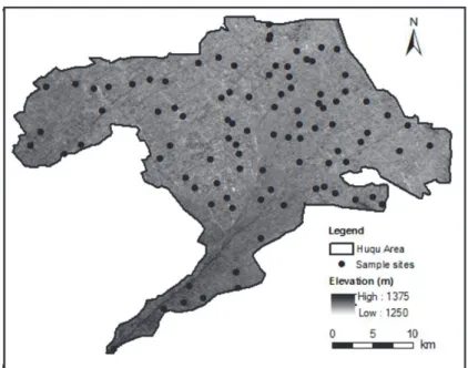
Fig. 5 Locations of the 94 soil samples analyzed in the present study

2.2.2 Soil sampling

The field dataset was obtained during April 2015, when the salt concentration in surface soils reaches its maximum in this region. In April, the low precipitation combines with a high evaporation rate to cause salt from deeper soil layers to migrate upwards and accumulate near the surface of the soil (Elnaggar and Noller, 2009). We obtained 94 surface soil samples (Fig. 2-b) to a depth of 10 cm from unused land ( 9 samples from shrubland, 5 samples from abandoned land, 46 samples from sparse grassland, 13 samples from saline wasteland) and cropland (used to grow wheat, sunflower, alfalfa, goji berry, and fennel). The sites were selected based on the results of previous soil salinity studies and Google Earth images, and each sample site represented an area of 90 m ×90 m. For each sample point, we combined five topsoil samples into a single composite sample, which we used to represent the value of the soil chemical parameters at that site. The location of each sample point was recorded with a MAP64SJZ GPS receiver (Garmin, Olathe, KS, USA) and we photographed the site. The characteristics of the soil surface, the landuse and cover types surrounding the site, and the vegetation cover were recorded in a field notebook. We also consulted local farmers to learn about historical land use and cover types.

(29)

2.2.3 Laboratory analysis

Soil moisture was assessed during the soil sample collection. The samples were sealed into weighed, empty specimen boxes and their total weights were measured.

When we returned to the laboratory, we opened the boxes and oven-dried the samples for 24 hours at 105 °C together with the boxes. We calculated the soil moisture content (SMC) as a percentage of the dry soil weight.

For the chemical analysis, the samples were air-dried, crushed, and passed through a 1-mm sieve to remove large particles and plant residues. To quantify the soil salinity, we measured the electrical conductivity (EC1:5) in deionized distilled water at 1:5 g/ml soil:water ratio. The standard methodology for the soil salinity assessment needs to measure the EC from the soil saturated paste extract, which is cumbersome and tedious. One of the most widely used soil over water mass ratios is 1:5. An Investigation of the relationship between the ECe with the EC1:5

for soils in Greece showed that the mean ECe is about 6.5 times larger than EC1:5 with a linear model of ECe = 6.5318 EC1:5 - 0.1088 (R^² = 0.9317) (George K. et al., 2018).

However, the coefficients of their relationship vary according to the area of interest.

We calculated the frequency distribution of these values and several associated parameters: the mean, median, standard deviation, skewness, kurtosis, range, and maximum and minimum values. We used version 23 of the SPSS software (www.ibm.com/analytics/us/en/technology/spss/) for our statistical analysis.

We also measured the soil pH. To make the pH measurements better reflect the water content of the soil under field conditions, we used a 1:1 g/ml soil solution (Thomas G.W. et al., 1996).

2.2.4 GIS and map preparation

Maps of the distribution of soil EC1:5 were prepared to visualize the results at the 94 sample sites. We used version 10.2.1 of the ArcView software (www.esri.com). We also visualized the layout of the irrigation canal network, depths to the water table, and

(30)

20

TDS data for the water using ArcView. Additional data included an ASTER Global Digital Elevation Model (ASTER GDEM) acquired from https://gdex.cr.usgs.gov/gdex/ at a 30-m resolution. To describe the topographic characteristics of the sample sites, we derived the compound topographic index (CTI), which is widely used in hydrology and terrain-related applications, from the ASTER GDEM data (Beven and Kirkby, 1979). CTI is a compound index that is calculated using two primary topographic attributes ( Moore I.D., Grayson R.B. and Ladson A.R, 1991); it is also known as the steady-state wetness index when it is used to quantify the catenary landscape position ( Gessler et al., 2000). The following equation was used to calculate the CTI values

CTI = ln ( (1)

Low CTI values represent small catchments, steep slopes, and upper catenary positions.

High CTI values represent large catchments, gentle slopes, and lower catenary positions with a higher capacity for water accumulation and wetness (Marthews, T.R., 2015).

2.2.5 Grey relational analysis

A grey relationship is a relationship among different types of data series often with different units of measurement when there is considerable uncertainty and an unsatisfactory sample size (Huang J., 2011). Grey relational analysis (GRA) is a way to identify the key factors that control a system and quantify the influence that each factor exerts on a reference variable (Lin S. J. et al., 2007). It is often applied in studies that have an insufficient sample size and uncertainty about whether the data is truly representative (Kayacan et al., 2010; Huang J., 2011). The basic idea behind GRA is to compute the strength of the relationship between variables by examining the degree of proximity for certain geometrical or the degree of correlation between curves (Deng, 1989). In this study, we employed GRA to quantify the influence of several factors on the soil salinity of the 94 samples from the Huqu area.

(31)

In GRA, the original data series are divided into two types of series: a reference series that will be compared with all other variables and one or more affecting series (one per variable that potentially affects the values in the reference series). The grey strength of the relationship is calculated to represent the relative proximity of twoseries.

A discrete sequence of ranks can then be generated, with the ranks depending on the

relationship for one affecting series is higher than that of the others, the former series is considered to have a greater influence than the others on the reference series (Deng, 1989).

The first step in GRA is to generate the reference series and the affecting series.

Since the range of values and the units of measurement in one data series may differ from those in other series, the original data are first normalized by dividing each value by the maximum value in the series, thereby producing a range of values from 0 to 1, and are then used to calculate the grey relational coefficient between the reference series and the affecting series (Sallehuddin R., et al., 2008). The reference series is represented

as (1,

xi(1), xi

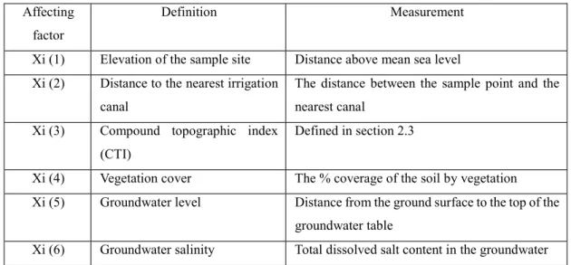
soil EC1:5 (dS/m) as the reference series. Based on our review of the research literature and the mechanisms of salinization, as well as based on data availability, we selected six affecting factors for use as the affecting series (Table 3).

(32)

22

Table 3 Definitions of the affecting factors for the reference series (soil EC1:5) Affecting

factor

Definition Measurement

Xi (1) Elevation of the sample site Distance above mean sea level Xi (2) Distance to the nearest irrigation

canal

The distance between the sample point and the nearest canal

Xi (3) Compound topographic index (CTI)

Defined in section 2.3

Xi (4) Vegetation cover The % coverage of the soil by vegetation Xi (5) Groundwater level Distance from the ground surface to the top of the

groundwater table

Xi (6) Groundwater salinity Total dissolved salt content in the groundwater

The grey relational coefficient for two

(2)

Where xi(k)| is the absolute difference between the reference factor x0(k) and the corresponding affecting factor xi(k);

value between 0 and 1, and that is often assigned a value equaled 0.5, a value that is commonly used (Song, S., et al., 2011) represent the smallest and biggest values, respectively, among all of the .

and the reference series x0(k) can be calculated by averaging the grey relational coefficient corresponding to each affecting factor:

) (3)

The ranking of the affecting factors is then conducted based on the computed grey relational grades. As mentioned earlier, a higher value of the grey relational grade indicates a stronger relationship between the two series and suggests that the corresponding affecting factor is closer to the reference series than other affecting factors (Gao et al., 2013)

(33)

2.3 Results and discussions

2.3.1 Statistical description

Fig. 6 shows the frequency distribution and descriptive statistics for EC1:5 of the cropland and other land types. 21 soil samples were collected from cropland during the spring, which explains why many samples have a low EC1:5 value. 73 soil samples were collected from other land types (shrubland, abandoned land, sparse grassland and saline wasteland). Fig. 6 also shows wide variation in the EC1:5 data, with values ranging from 0.11 to 23.1 dS/m (two orders of magnitude).

Fig. 6 Histograms of EC1:5 values for samples from (a) cropland (n = 21) and (b) all other land types (n = 73), and their associated descriptive statistics

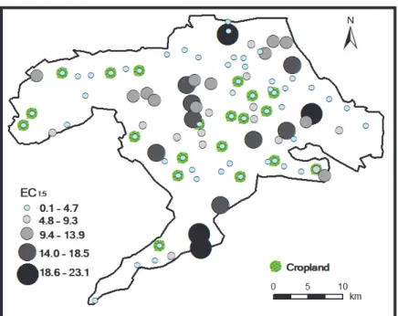
To understand the spatial distribution of the salinity levels, we mapped the distribution of soil EC1:5 using ArcView based on equal interval method (Fig. 7). As the distribution map shows, most of the samples with high EC1:5 were distributed at the margins of the oasis, but some were distributed in the center; in contrast, the samples with lower EC1:5 were distributed throughout the oasis.

(34)

24

Fig. 7 Map of the distribution of EC1:5 values for the 94 soil samples.

2.3.2 Differences in soil salinity among the different land use and cover types

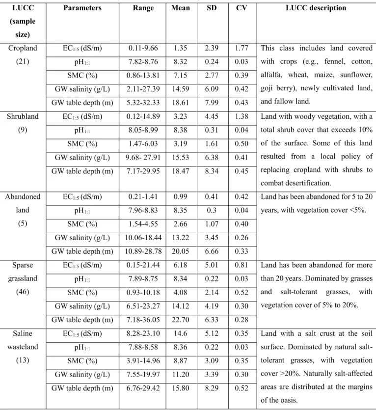
To further explore the characteristics of the distribution of the soil EC1:5 values in the Huqu area in relation to the land management in the study area, we classified the 94 samples into the five main land use and cover types: cropland, shrubland, abandoned land, sparse grassland, and saline wasteland. Table 2 summarizes the measured values of the various properties of the soil samples.

The coefficient of variation (CV) is the ratio of the standard deviation to the mean, and is often used as a general index of variability among the samples (Wilding and Drees, 1983). A CV value lower than 0.1 (10%) indicates low variability, whereas a CV value higher than 1.0 (100%) indicates high variability; intermediate values have moderate variability (Adhikari et. al, 2011). Table 4 shows that the CV values of EC1:5

for cropland and shrubland were highly variable, with CV values greater than 1.0, which suggests that EC1:5 and its distribution pattern are strongly influenced by human driving factors such as irrigation and farming activities as well as by the irrigation canal system.

Despite regular irrigation, some of the cropland soil EC1:5 values reached 9.66 dS/m, which indicates the existence of a secondary salinization problem. The shrubland is

(35)

mainly artificial, and has resulted from a local policy to replace cropland with shrubs to combat desertification. The low soil moisture content of the shrubland provides evidence of a water scarcity problem. This is consistent with previous research, which showed that shrubs have died in large areas because the groundwater level fell below the level their roots can reach. The maximum EC1:5 value of shrubland reached 14.89 dS/m, which indicated large amounts of salt accumulation in the topsoil as a result of a high evaporation rate combined with low rainfall and mineralization of the groundwater.

The CV values of EC1:5 for abandoned land, sparse grassland, and saline wasteland were moderate (between 0.1 and 1.0). These land use and cover types were less strongly affected by human activities. Abandoned land was defined as land that had been abandoned for 5 to 20 years, and sparse grassland has been abandoned for more than 20 years and has begun to develop a grassland ecosystem. The majority of the soil EC1:5

values for abandoned land were lower than those for sparse grassland, which indicated that soil salinity increased with increasing duration of abandonment. Compared with sparse grassland, the salinity level and moisture content of soils in the abandoned land were lower.

The CV values for SMC for all land use and cover types showed moderate variability (0.1 to 1.0). The pH1:1 of the soil of the study areas ranged from 7.82 to 8.99 (slightly alkaline), and its low CV values (<0.1) indicated slight variation. The mean pH1:1 for all land use and cover types was greater than 8, which indicated most of the soil samples are weakly alkaline. The high groundwater salinity (>11 g/L) content and deep groundwater table depth (>15 m) indicated poor water quality and poor access to water, and their low CV values indicate moderate spatial variability.

(36)

26

Table 4 Descriptive statistics for the soil parameters, by land use and cover class (LUCC)a LUCC

(sample size)

Parameters Range Mean SD CV LUCC description

Cropland (21)

EC1:5 (dS/m) 0.11-9.66 1.35 2.39 1.77 This class includes land covered with crops (e.g., fennel, cotton, alfalfa, wheat, maize, sunflower, goji berry), newly cultivated land, and fallow land.

pH1:1 7.82-8.76 8.32 0.24 0.03

SMC (%) 0.86-13.81 7.15 2.77 0.39 GW salinity (g/L) 2.11-27.39 14.59 6.09 0.42 GW table depth (m) 5.32-32.33 18.61 7.99 0.43 Shrubland

(9)

EC1:5 (dS/m) 0.12-14.89 3.23 4.45 1.38 Land with woody vegetation, with a total shrub cover that exceeds 10%

of the surface. Some of this land resulted from a local policy of replacing cropland with shrubs to combat desertification.

pH1:1 8.05-8.99 8.38 0.31 0.04

SMC (%) 1.47-6.03 3.19 1.61 0.50 GW salinity (g/L) 9.68- 27.91 15.53 6.38 0.41 GW table depth (m) 7.17-29.95 18.47 8.34 0.45

Abandoned land

(5)

EC1:5 (dS/m) 0.21-1.41 0.99 0.41 0.42 Land has been abandoned for 5 to 20 years, with vegetation cover <5%.

pH1:1 7.96-8.83 8.35 0.3 0.04

SMC (%) 1.54-4.55 2.66 1.07 0.40 GW salinity (g/L) 10.06-18.44 13.22 3.45 0.26 GW table depth (m) 10.89-28.78 20.05 6.66 0.33 Sparse

grassland (46)

EC1:5 (dS/m) 0.15-21.44 6.18 5.01 0.81 Land has been abandoned for more than 20 years. Dominated by grasses and salt-tolerant grasses, with vegetation cover of 5% to 20%.

pH1:1 7.89-8.75 8.34 0.22 0.03

SMC (%) 0.93-10.18 4.08 2.14 0.52 GW salinity (g/L) 6.51-23.27 14.12 4.19 0.30 GW table depth (m) 7.18-36.05 22.70 6.33 0.28 Saline

wasteland (13)

EC1:5 (dS/m) 8.28-23.10 14.6 5.12 0.35 Land with a salt crust at the soil surface. Dominated by natural salt- tolerant grasses, with vegetation cover >20%. Naturally salt-affected areas are distributed at the margins of the oasis.