Central limit theorems for non-symmetric random walks on covering graphs

(1)

Central limit theorems for non-symmetric random walks on covering graphs

Doctoral thesis presented by

Ryuya NAMBA to

Graduate School of Natural Science and Technology Okayama University

Okayama, Japan

March 2019

(2)

(3)

Acknowledgements

I have been extremely happy to get encouragements and supports from a number of people and institutions. Thanks to all of them, I can continue to enjoy mathematics and can complete my work in the form of this thesis. Let me give an opportunity to express my gratitude and indebtedness to all those who have been helped me.

First and foremost, I would like to express my great appreciation to Professor Hiroshi Kawabi. He led me to a vast world of probability theory and provided me with insightful guidance and great encouragement throughout my study on long time behaviors of random walks on covering graphs. His wide and deep knowledge was enough to stimulate my mathematical curiosity.

I am grateful to Professor Satoshi Ishiwata for fruitful discussions through our jointwork served as a foundation for this thesis, and for telling me the ideal attitudes to mathematics in every respect.

I would like to thank Professor Kazuyoshi Kiyohara for kindly agreeing to be the chair of the examination board. I also thank Professors Takahiro Aoyama and Seiichiro Kusuoka for reading the early versions of my preprints very carefully and for providing me with valuable comments, to say nothing of supporting my PhD studies at Okayama University in many respects. I am very grateful to Professor Shoichi Fujimori for making very beautiful figures and animations of the three-dimensional Heisenberg dice lattice and kindly allowing me to use them in my papers.

Special thanks are owed to Professors Massimiliano Gubinelli and Peter K. Friz, who provided me chances of research visits at Universität Bonn, Germany in March 2017 and Technische Universität Berlin, Germany in November 2018, respectively. Professor Gubinelli gave me much insightful and valuable advice on rough paths, which improved my results dramatically. I also would like to thank Research Institute for Interdisciplinary Science, Okayama University for supporting my one-month research stay at Universität Bonn. Professor Friz helped me find new possible directions of my research and gave me an opportunity to talk in Weekly Seminar on rough paths, stochastic partial differential equations and related topics at Technische Universität Berlin.

I would like to express my sincere gratitude to Professors Takafumi Amaba, Naotaka Kajino, Atsushi Katsuda, Takashi Kumagai, Kazumasa Kuwada, Laurent Saloﬀ-Coste, Yuichi Shiozawa and Ryokichi Tanaka, and Dr. Kohei Suzuki for helpful discussions and encouragements.

I was partially supported by Japan Society for the Promotion of Science, Research

(4)

Fellowships for Young Scientists, Number 18J10225.

Finally, and most importantly, I would like to thank my family for support and encouragement, without which this thesis would not have been written. To my family, I dedicate this thesis.

Ryuya Namba

4

(5)

Chapter 1 Introduction

Random walks are one of the most fundamental classes of stochastic processes and well- studied topics in harmonic analysis, geometry, graph theory and group theory, to say nothing of probability theory. These are defined to be time-homogeneous Markov chains whose transition probability is adapted to the structures of the underlying state space.

From the probabilistic and geometric perspectives, many authors have been tried to study long time asymptotics of random walks in various settings. In particular, a central limit theorem (CLT), that is, a generalization of the Laplace–de Moivre theorem, must be a central problem and is studied intensively and extensively. Roughly speaking, the CLT asserts that the limiting distribution of random walks under an appropriate scaling of space and time is nothing but the normal distribution. Furthermore, a functional CLT (Donsker’s invariance principle) is well-known as a stronger assertion and it means that the distribution of a corresponding rescaled path-valued process converges to that of Brownian motion. These mathematical backgrounds basically motivate author’s study.

For the classical results on random walks, see Spitzer [66]. We refer to Woess [79] for rich results on random walks on infinite state spaces with extensive references therein.

See also Lawler–Limic [48] for relation between random walks and potential theory and Barlow [5] for properties of heat kernels of random walks.

Our main concerns of this thesis are long time asymptotics of random walks on infinite graphs. In particular, we pay much attention to geometric features of the graph such as the periodicity and the volume growth, which play important role to obtain the asymptotics (see e.g., Spitzer [66] and Woess [79]). A covering graph of a finite graph, which is a discrete analogue of covering spaces, is a basic and typical example equipped with the above two geometric features. In this study, we usually employ ideas from the method of homogenization. Generally speaking, homogenization theory is a method which relates a periodic system to the corresponding homogenized system through a scaling relation between the time and the underlying state space (cf. Bensoussan–Lions–Papanicolaou [8]).

However, since the notion of the scale change on graphs is not defined, it is not possible to apply this method directly to the case where the underlying space is an infinite graph.

Therefore, it is necessary to find a realization of the graph, preserving the geometric

(8)

features, in a space on which a scaling is defined.

We now focus on an infinite graph which is equipped with the periodicity. A typical example of such infinite graphs is a crystal lattice, that is, a covering graph X of a finite graph X₀ whose covering transformation group Γ is finitely generated and abelian. It is regarded as a generalization of the square lattice, the triangular lattice, the hexagonal lattice, the dice lattice and so on (see Figure 1.1). We remark that the crystal lattice has

Square lattice Triangular lattice

X0= X0=

σ1

σ2

σ1

σ2

Hexagonal lattice

X0= σ1

σ2

Dice lattice

X0= σ1

σ2

1

Figure 1.1: Crystal lattices with the covering transformation group Γ =⟨σ₁, σ₂⟩ ∼=Z² inhomogeneous local structures though it has a periodic global structure. Let us briefly review the history of the study of random walks on crystal lattices. In Kotani–Shirai–

Sunada [43], an asymptotic behavior of the n-step transition probability of symmetric random walks on crystal lattices was obtained. As mentioned above, there is an essential diﬃculty to establish CLTs for random walks on crystal lattices, because such a graph does not have any appropriate spatial scaling. In order to overcome this diﬃculty, Kotani and Sunada [41] introduced the notion ofstandard realizationof a crystal latticeX, which is a discrete harmonic map Φ₀ from X into the Euclidean space Γ⊗R equipped with the Albanese metricassociated with the given transition probability. It characterizes an equi- librium configuration of X in a geometric point of view. In Kotani–Sunada [40], they discussed the relation between the standard realization ofX and the CLT for symmetric random walks on X. As the scaling limit, they captured a homogenized Laplacian on Γ⊗R. In terms of probability theory, it means that, for fixed 0 ≤ t ≤ 1, a sequence of Γ⊗R-valued random variables {n⁻^1/2Φ₀(w_[nt])}^∞n=1 converges to B_t asn → ∞ in law.

Here {w_n}^∞n=0 is the given symmetric random walk on X and (B_t)₀_≤_t_≤₁ is a standard 8

(9)

Brownian motion on Γ⊗R equipped with the Albanese metric. In their proof, both the symmetry of the given random walk {w_n}^∞n=0 and the harmonicity of the realization Φ₀ play an important role to show the convergence of the sequence of infinitesimal generators associated with {n⁻^1/2Φ0(w_[nt]) : 0≤ t ≤1}^∞n=1. Indeed, these properties are eﬀectively used to delete a diverging drift term asn → ∞from the homogenized Laplacian. See also Kotani [38] for the proof of CLT for magnetic transition operator onX via this technique.

Moreover, Kotani and Sunada [42] obtained the large deviation principle (LDP) for random walks on X (see also Section 2.6). Among these papers, they developed a hybrid field of several traditional disciplines including graph theory, geometry, discrete group theory and probability theory. Since this new field, called discrete geometric analysis, was introduced by Sunada, it has been making new interactions with many other fields.

For example, Le Jan employed discrete geometric analysis eﬀectively in a series of recent studies of Markov loops (see e.g., [49, 50]). We refer to Sunada [70, 71] for recent progress of discrete geometric analysis.

On the other hand, it turns out that the notion of volume growth aﬀects the long time asymptotics of random walks on finitely generated groups or Cayley graphs of them.

Suppose a finitely generated group Γ with the generating set {γ₁^±¹, γ₂^±¹, . . . , γ_ℓ^±¹}satisfies

#{γ_k^ε₁¹γ_k^ε₂². . . γ_k^εⁿ_n|ki = 1,2, . . . , ℓ, εi = 1,−1, i= 1,2, . . . , n} ≤C·V(n) (n ∈N) for some constant C > 0 and some function V(n). If V(n) ≤ n^d(n ∈ N) for some d ∈ N, then we call Γ a group of polynomial volume growth. Otherwise, we call it a group ofsuperpolynomial volume growth. Generally, it is difficult to characterize a finitely generated group itself in terms of its volume growth. For example, all non-amenable groups haveexponentialvolume growth, however there are also many amenable groups of exponential volume growth. In fact, this kind of difficulty comes from the diversity and complexity of the algebraic structures of finitely generated groups. We refer to Saloff- Coste [65] for basic problems and results for random walks on such groups including the case of superpolynomial volume growth. On the contrary, there is a remarkable theorem on a group of polynomial volume growth due to Gromov, which asserts that it is essentially characterized as a nilpotent group (cf. Gromov [25] and Ozawa [59]). Hence, we find a large number of papers on long time asymptotics of symmetric random walks on state spaces with a nilpotent structure. We refer to Wehn [78], Tutubalin [75] and Stroock–

Varadhan [68] for related early works, Raugi [63], Pap [61], Watkins [77] and Alexopoulos [3] for CLTs for centered random walks on nilpotent Lie groups. See also Breuillard [10] for an overview of random walks on Lie groups with extensive references. For local CLTs on nilpotent Lie groups, Alexopoulos [1, 2], Breuillard [11], Diaconis–Hough [17] and Hough [28] may be consulted.

In view of these developments, it is natural to ask whether the long time asymptotic of random walks on a covering graphX whose covering transformation group Γ is a finitely generated group of polynomial volume growth is obtained or not. The graphXis regarded as a generalization of a crystal lattice or the Cayley graph of a finitely generated group

(10)

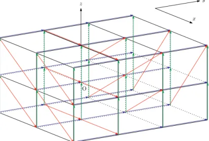
of polynomial volume growth. A typical example of such Γ is the 3-dimensional (3D) discrete Heisenberg group Γ = H³(Z) (see Figure 1.2). Thanks to Gromov’s theorem mentioned above, Γ has a finite extension of a torsion free nilpotent subgroup eΓ◁Γ.

Therefore, X is regarded as a covering graph of the finite quotient graph eΓ\X whose covering transformation group isΓ. Hence, we may assume thate X is a covering graph of a finite graph X₀ whose covering transformation group Γ is a finitely generated, torsion free nilpotent group of step r (r ∈ N) without loss of generality. We now mention a few related works on long time asymptotics of random walks on a Γ-nilpotent covering graph X. Ishiwata [29] discussed symmetric random walks on X and extended the notion of standard realization of crystal lattices to the nilpotent case, so that the similar problems to the case of crystal lattices could be considered. As a result, a semigroup CLT was obtained through the standard realization Φ₀ of X into a nilpotent Lie group G=G_Γ such that Γ is isomorphic to a cocompact lattice in G equipped with a scalar multiplication called a one-parameter family of canonical dilations (τ_ε)_ε>0 (cf. Malc´ev [56]). More precisely, he captured the homogenized sub-Laplacian on G associated with the Albanese metric on g⁽¹⁾ as the CLT-scaling limit. Here g⁽¹⁾ stands for the generating part of the Lie algebra g of G. We note that the diverging drift term appears only in g⁽¹⁾-direction due to the basic property of the dilation operator. Hence, it is suﬃcient to introduce the notion of harmonicity of the realization Φ₀ only on g⁽¹⁾ for proving the CLT in the nilpotent case.

In spite of such developments, long time asymptotics ofnon-symmetric random walks on nilpotent covering graphs have not been studied suﬃciently though an LDP on X was obtained in Tanaka [72] (see also Section 2.6).

Case.2 ,Γ Cayley X= (V, E)

. ,Γ γ1,γ2,γ3

γ1=

⎛

⎜⎝ 1 1 0 0 1 0 0 0 1

⎞

⎟⎠, γ2=

⎛

⎜⎝ 1 0 0 0 1 1 0 0 1

⎞

⎟⎠, γ3=

⎛

⎜⎝ 1 0 1 0 1 0 0 0 1

⎞

⎟⎠

.γ1,γ2,γ3 2 ,

γ1←→(1,0,0), γ2←→(0,1,0), γ3←→(0,0,1) γ₁⁻¹←→(−1,0,0), γ₂⁻¹←→(0,−1,0), γ⁻¹₃ ←→(0,0,−1)

.

z y

x

O

12 : Heisenberg Γ Cayley , 2.

,γ1,γ2,γ3 exp⁻¹:GΓ−→g , . exp⁻¹(γ1) =X¹, exp⁻¹(γ2) =X², exp⁻¹(γ3) =X³.

Γ Cayley X .g= (x, y, z)∈Γ ,

γ1g= (x+ 1, y, z+y), γ2g= (x, y+ 1, z), γ3g= (x, y, z+ 1), γ⁻₁¹g= (x−1, y, z−y), γ₂⁻¹g= (x, y−1, z), γ⁻₃¹g= (x, y, z−1).

12 Cayley X . O Γ 1Γ↔(0,0,0) .

74

Figure 1.2: A part of the Cayley graph of Γ =H³(Z)

If we consider the non-symmetric case, the same method as the symmetric case does not work well for proving CLTs because the diverging drift term arising from the non- symmetry of the given random walk does not vanish. To overcome this diﬃculty, Ishiwata,

10

(11)

Kawabi and Kotani [31] introduced two kinds of schemes for proving functional CLTs (FCLTs) for a non-symmetric random walk {w_n}^∞n=0 on a crystal lattice X. One is to replace the usual transition operator by the transition-shift operator, which “deletes”

the diverging drift term. Combining this scheme with a modification of the harmonicity of the realization Φ₀, they proved that a sequence {

n⁻^1/2(

Φ₀(w_[nt]) −[nt]ρ_R(γ_p))

; 0 ≤ t ≤ 1}_∞

n=1 converges in law to a Γ ⊗ R-valued standard Brownian motion (B_t)_t_≥₀ as n → ∞. Here ρ_R(γ_p) ∈ Γ ⊗R is the so-called asymptotic direction which appears in the law of large numbers for the random walk {Φ₀(w_n)}^∞n=0 on Γ⊗R (see Proposition 2.5.1). The other is to introduce a one-parameter family of Γ⊗R-valued random walks (ξ^(ε))0≤ε≤1 which “weakens” the diverging drift term, where this family interpolates the original non-symmetric random walkξn⁽¹⁾ := Φ₀(w_n) (n = 0,1,2, . . .) and the symmetrized one ξ⁽⁰⁾. Putting ε = n^−1/2 and letting n → ∞, we capture a drifted Brownian motion (B_t+ρ_R(γ_p)t)₀_≤_t_≤₁as the limit of a sequence{

n⁻^1/2ξ_[nt]⁽ⁿ⁻^1/2⁾; 0≤t≤1}_∞

n=1. See Trotter [74]

for related early works. It is worth mentioning that this scheme is well-known in the study of the hydrodynamic limit of weakly asymmetric exclusion processes. See e.g., Kipnis–

Landim [36], Tanaka [72] and references therein. In Alexopoulos [2], a non-centered random walk on a finitely generated group of polynomial volume growth Γ is discussed.

For the same reason as above, in the non-centered case, the diverging drift term prevents us from obtaining CLTs. He introduced another kind of scheme to avoid this problem. It is to establish a measure-change formula for the given non-centered transition probability on Γ, to “change” the situation into the drftless one. We note that it corresponds to a kind of Girsanov’s formula on Γ. As an application of this scheme, he proved a CLT and a generalization of the Berry–Esseen type estimate for non-centered random walks on Γ.

The main purpose of this thesis is to investigate long time asymptotics of non-symmetric random walks on covering graphs in view of the three schemes explained above. We now state frameworks and results with the organization of this thesis.

Chapter 2: We lay the foundations that will be needed in all subsequent chapters. We give several definitions, notations and properties of graphs and random walks, as well as those of function spaces on a metric space in Section 2.1. We review basic materials on nilpotent Lie groups and corresponding Lie algebras in Section 2.2. In particular, the notion of limit group of a nilpotent Lie group is introduced, which is defined by a certain deformation of the original Lie-group product through the dilation operator. Note that it plays a very important role to establish main results in Chapters 4 and 5. Section 2.3 concerns with two notions on nilpotent Lie groups. One is the Carnot–Carath´eodory metric, which is an intrinsic metric appeared in the context of sub-Riemannian geometry.

The other is homogeneous norms, which is compatible with dilations and behaves like a

“norm” on G. In Section 2.4, we summarize the theory of discrete geometric analysis on finite graphs which was developed by Kotani and Sunada. After that, we apply the theory to introduce the notion of modified harmonic realization of both a crystal lattice and a nilpotent covering graph (Definitions 2.4.5 and 2.4.6). As is well-known, there is an important relation between the notion of martingale and that of harmonicity. In Section

(12)

2.5, such relations for Markov chains with values in both a crystal lattice and a nilpotent covering graph are clearly stated (Lemmas 2.5.1 and 2.5.3). Finally, in Section 2.6, we summarize the known results on LDP on covering graphs due to Kotani–Sunada [42, 39]

and Tanaka [72], with a relation between the LDPs and geometric aspects such as the Gromov–Hausdorﬀ limit of scaled covering graphs.

Chapter 3: The content of this chapter is based on author’s paper [58], discussing a measure-change formula for non-symmetric random walks on a Γ-crystal lattice X. In Section 3.1, we establish the measure-change formula by using a variational method due to Alexopoulos [2]. We introduce a functionF :X₀×Hom(Γ,R)−→Rby (3.1.1), where X₀ = Γ\X is the quotient graph. We show that, for a fixed vertex x ∈ X₀, there exists a unique minimizer λ_∗ =λ_∗(x)∈Hom(Γ,R) of the function F (Lemma 3.1.1). By using this minimizer λ_∗(x), we then construct a new transition probability p on the crystal lattice such that it is still non-symmetric but the asymptotic direction ρ_R(γ_p) vanishes (see (3.1.4) for the definition). This means that, under the new transition probability p, the modified harmonic realization Φ₀ is regarded as the harmonic realization. We apply the measure-change formula to give yet another approach to the proof of CLTs (Lemma 3.2.3 and Theorem 3.2.1) for non-symmetric random walks on a crystal lattice in Section 3.2. More precisely, we show that, in a H¨older space over Γ⊗R, a sequence {n⁻^1/2Φ0(w_[nt]^(p)) : 0 ≤ t ≤ 1}^∞n=1 converges in law to a Γ⊗R-valued standard Brownian motion (B_t)₀_≤_t_≤₁ as n → ∞. Here {w^(p)n }^∞n=0 is the random walk on X governed by the changed transition probabilityp. In the proof, the diverging drift term vanishes thanks to the (p-)harmonicity of the realization Φ₀. Moreover, an asymptotic relation between the given n-step transition probability and the changed one is also discussed (see Theorem 3.2.5). The measure-change formula is regarded as a discrete analogue of Girsanov’s formula, which is well-studied in stochastic analysis. Indeed, in Fujita [23], a discrete Girsanov’s formula for non-symmetric random walks on Z¹ was established. We discuss a relation between our formula and the above Girsanov’s formula in the case where the quotient graph is a bouquet graph in Section 3.3.

Chapter 4: This chapter is based on author’s paper [32], which is jointwork with Satoshi Ishiwata and Hiroshi Kawabi. We establish CLTs for non-symmetric random walks on a Γ-nilpotent covering graph X by using the transition-shift scheme mentioned above. We give settings and statements of main results in Section 4.1. Let Φ₀ : X −→ G =G_Γ be the modified standard realization of X, where the Lie algebragofGis equipped with the Albanese metric. Since the modified harmonicity of Φ₀ is defined only ong⁽¹⁾, we remark that the modified harmonic realization Φ₀ has the ambiguity except for the component corresponding to g⁽¹⁾. Through the map Φ₀, in Section 4.2, we obtain a semigroup CLT (Theorem 4.1.2), which means that the n-th iteration of the “transition shift operator”

converges to a diﬀusion semigroup on G as n → ∞ with a suitable scale change on G. The infinitesimal generator −A of the diﬀusion semigroup is the homogenized sub- Laplacian with a non-trivialg⁽²⁾-valued driftβ(Φ₀) arising from the non-symmetry of the given random walk, where g⁽²⁾ := [g⁽¹⁾,g⁽¹⁾]. The drift β(Φ₀) seems to depend on the

12

(13)

choice of a modified harmonic realization Φ₀ due to the g⁽²⁾-ambiguity mentioned above.

On the contrary, we show that it is independent of the choice of Φ₀ (Proposition 4.2.3).

Furthermore, by imposing an additional natural condition (C), we prove an FCLT in a Hölder space over G (Theorem 4.1.3) in Section 4.3. Note that the FCLT is much stronger than Theorem 4.1.2. Roughly speaking, we capture aG-valued diffusion process associated with−A through the CLT-scaling limit of the non-symmetric random walk on X. We call the condition(C) the centered condition. As is emphasized in Breuillard [10, Section 6], the situation of the non-centered case is quite different from the centered case and thus some technical difficulties arise to obtain CLTs. That is why there are few papers which discuss CLTs for non-centered random walks on nilpotent Lie groups. We obtain, in Theorem 4.1.2, a semigroup CLT for the non-centered random walk{ξ_n := Φ₀(w_n)}^∞n=0

on G with a canonical dilation τ_n−1/2, while Cr´epel–Raugi [15] and Raugi [63] proved similar CLTs for the random walk to (4.1.6) with spatial scalings whose orders are higher than τ_n−1/2. On the other hand, we need to assume the centered condition(C) to obtain an FCLT (Theorem 4.1.3) for {ξ_n}^∞n=0 in the H¨older topology, which is stronger than the uniform topology. In Section 4.4, we extend the measure-change method established in Section 3 to the nilpotent case and establish a CLT and an FCLT (Theorems 4.4.2 and 4.4.3) as generalizations of Theorems 4.1.2 and Theorem 4.1.3.

Let us give another motivation of this study from rough path theory, which will be discussed in Section 4.5. It is known that rough path theory was initiated by Lyons in [54]

to discuss line integrals and ordinary diﬀerential equations (ODEs) driven by an irregular path such as a sample path of Brownian motionB = (B_t)₀_≤_t_≤₁ onR^d. Rough path theory makes us possible to handle a Stratonovich type stochastic diﬀerential equation (SDE) driven by Brownian motion B as a deterministic ODE driven by standard Brownian rough path (i.e., Stratonovich enhanced Brownian motion) B = (B,B), where B is a couple of Brownian motion B itself and its Stratonovich iterated integralB. Thus, rough path theory provides a new insight to the usual SDE-theory and it has developed rapidly in stochastic analysis. For more details on an overview of rough path theory and its applications to stochastic analysis, see Lyons–Qian [55], Friz–Victoir [22] and Friz–Hairer [19]. In the rough path framework, several authors have studied Donsker-type invariance principles. Among them, Breuillard–Friz–Huesmann [12] first studied this problem for Brownian rough path. Namely, they captured Stratonovich enhanced Brownian motion B = (B,B) on R^d as the usual CLT-scaling limit of the natural rough path lift of an R^d-valued random walk with the centered condition. We also refer to Bayer–Friz [6]

for applications to cubature and Chevyrev [14] for a recent study on an extension to the case of L´evy processes. Here we should note that there are good approximations to Brownian motion which do not converge to B but instead to a distorted Brownian rough pathB= (B,B+β), whereβis an anti-symmetric perturbation of B. For example, Friz–

Gassiat–Lyons [18] constructed such a rough path called magnetic Brownian rough path as the small mass limit of the natural rough path lift of a physical Brownian motion onR^d in a magnetic field. Through this approximation, they showed an eﬀect of the magnetic

(14)

field appears explicitly in the anti-symmetric perturbation term β. See also e.g., Lejay–

Lyons [51] and Friz–Oberhauser [21] for related results on this topic. In view of the background described above, we discuss a random walk approximation of the distorted Brownian rough path B from a perspective of discrete geometric analysis. Since the unique Lyons extension of B of orderr (r ≥2) can be regarded as a diffusion process on a free step-r nilpotent Lie group G^(r)(R^d), we obtain such a diffusion process in Corollary 4.5.4 through the CLT-scaling limit of a non-symmetric random walk on a nilpotent covering graph X as a direct application of Theorem 4.1.3. Besides, we observe that the non-symmetry of the random walk on X affects the anti-symmetric perturbation term of B explicitly. Recently, Lopusanschi–Simon [53] and Lopusanschi–Orenshtein [52] proved a similar invariance principle for B to ours. However, they did not discuss an explicit relation between the perturbation term, called the area anomaly, and the non-symmetry of the given random walk. In view of that, Corollary 4.5.4 gives a new approach to such an invariance principle in that we pay much attention to the non-symmetry of random walks on X.

Finally, in Section 4.6, we concern with an FCLT for a non-symmetric random walk {w_n}^∞n=0 on X through a non-harmonic realization Φ : X −→ G, though the modified harmonicity of realizations play an important role in the proof of the FCLT (Theorem 4.1.3). We employ the so-called corrector method, which is often used in the study of invariance principles on random media (see e.g., Kumagai [45]). By noting the definition of the (g⁽¹⁾-)modified harmonic realization Φ₀, we introduce the g⁽¹⁾-corrector of a non- harmonic realization Φ by the diﬀerence ofg⁽¹⁾-components of Φ and Φ₀. In fact, we notice that this corrector is easy to estimate thanks to the periodicity of these realizations.

By using the estimation, we show that, under the centered condition, the sequence of stochastic processes given by the geodesic interpolation of the G-valued scaled random walk{τ_n−1/2Φ(w_k)}ⁿk=0 also converges to the same diﬀusion as captured in Theorem 4.1.3.

See Theorem 4.6.2 for details.

Chapter 5: This chapter is based on author’s paper [33], which is jointwork with Satoshi Ishiwata and Hiroshi Kawabi. As a continuation of Section 4, we study another kind of CLTs for a non-symmetric random walk {w_n}^∞_n=0 on a Γ-nilpotent covering graph X by applying the scheme for weakening the diverging drift term. Settings and statements of main results are given in Section 5.1. We first introduce a one-parameter family of transition probabilities (pε)0≤ε≤1 onX as the linear interpolation between the given transition probability p₁ :=pand the symmetrized one p₀, that is, p_ε:=p₀+ε(p−p₀) (0≤ε≤1).

For each ε, we take a modified harmonic realization Φ^(ε)₀ : X −→ G associated with the transition probability p_ε, and define a one-parameter family of G-valued random walks (ξ^(ε))₀_≤_ε_≤₁ by ξn^(ε) := Φ^(ε)₀ (w_n) (n = 0,1,2, . . .). In Section 5.2, several properties of the family of modified harmonic realizations (Φ^(ε)₀ )₀_≤_ε_≤₁ are discussed. In the proof of a main result (Theorem 5.1.1), ag⁽²⁾-valued drift β(ε)(Φ^(ε)₀ ), which is likeβ(Φ0) in Section 4, will appear in the limiting infinitesimal generator and we need to know the behavior of it as ε ↘ 0. We show that the sequence of g⁽²⁾-valued drift vanishes as ε ↘ 0 under a

14

(15)

natural condition (A1). See Proposition 5.2.1. As a result, by putting ε = n⁻^1/2 and letting n → ∞, we prove a CLT (Theorem 5.1.1) for the family of G-valued random walks {ξ⁽ⁿ⁻^1/2⁾}^∞n=1 in Section 5.3. Furthermore, in Section 5.4, we show that a sequence {τ_n−1/2

(ξ⁽ⁿ_[nt]⁻^1/2⁾)

: 0 ≤ t ≤ 1}_∞

n=1 converges in law to a G-valued diffusion process as n → ∞ under suitable assumptions (A1) and (A2). See Theorem 5.1.2. Here the dif- fusion process is generated by the homogenized sub-Laplacian with the g⁽¹⁾-valued drift ρ_R(γ_p) defined on G equipped with the Albanese metric g⁽⁰⁾₀ associated with the symmetrized transition probability p₀. To our best knowledge, there seems to be few results on CLTs in the nilpotent setting in which a g⁽¹⁾-valued drift appears in the infinitesimal generator of the limiting diffusion. On the other hand, as we have already mentioned, there are many papers on CLTs in which g⁽²⁾-valued drift like β(Φ₀) appears in the infinitesimal generator of the limiting diffusion. In view of these circumstances, the study of the long time asymptotics of random walks on more general graphs by applying our

“weakening” scheme would be an interesting problem. In closing this section, we summarize the limiting infinitesimal generators and limiting diﬀusions captured in Chapters 4 and 5, as well as them on crystal lattices captured in Ishiwata–Kawabi–Kotani [31].

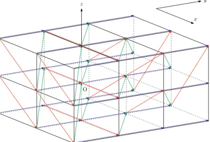
Chapter 6: This chapter is based on the author’s paper [32], which is jointwork with Satoshi Ishiwata and Hiroshi Kawabi. We give several concrete examples of non-symmetric random walks on Γ-nilpotent covering graphs in the case where Γ is the 3D discrete Heisenberg group H³(Z). We review some basics on H³(Z) in Section 6.1. We consider a non-symmetric random walk on the 3D Heisenberg triangular lattice (resp. the 3D Heisenberg dice lattice) in Section 6.2 (resp. in Section 6.3), as a generalization of the triangular lattice (resp. the dice lattice) to the nilpotent case. In both sections, explicit calculations on several quantities of random walks and several figures are given.

(16)

(17)

Chapter 2 Preliminaries

2.1 Notations

LetX = (V, E) be a locally finite, connected and oriented graph, where V is the set of all vertices andE is the set of all oriented edges. The graph X possibly have multiple edges or loops and is equipped with the discrete topology induced by the graph distance. For an edgee∈E, we denote by o(e) andt(e) the origin and the terminus ofe, respectively. The inverse edge of e∈E is defined by an edge, say e, satisfying o(e) =t(e) and t(e) =o(e).

Let E_x be the set of all edges whose origin is x ∈ V, that is, E_x = {e ∈ E|o(e) = x}. A path c in X of length n is a sequence c = (e₁, e₂, . . . , e_n) of n edges e₁, e₂, . . . , e_n ∈ E with o(e_i+1) = t(e_i) for i = 1,2, . . . , n−1. We denote by Ω_x,n(X) the set of all paths in X of lengthn ∈N∪ {∞}starting from x∈V. Put Ω_x(X) = Ω_x,_∞(X) for simplicity.

We introduce a transition probability, that is, a functionp:E −→[0,1] satisfying

∑

e∈Ex

p(e) = 1 (x∈V) and p(e) +p(e)>0 (e∈E).

The value p(e) represents the probability that a particle at the origin o(e) moves to the terminus t(e) along the edge e ∈ E in a unit time. The random walk associated with p is the X-valued time-homogeneous Markov chain (Ω_x(X),Px,{w_n}^∞n=0), where Px is the probability measure on Ωx(X) satisfying

Px

({c= (e₁, e₂, . . . , e_n,∗,∗, . . .)})

=p(e₁)p(e₂)· · ·p(e_n) (

c∈Ω_x(X)) and w_n(c) :=o(e_n+1) forn ∈N∪ {0} and c= (e₁, e₂, . . . , e_n, . . .)∈Ω_x(X).

We define the transition operatorL associated with the transition probability pby Lf(x) := ∑

e∈Ex

p(e)f( t(e))

(x∈V, f :V −→R) and then-step transition probability p(n, x, y) by

p(n, x, y) :=Lⁿδ_y(x) (n ∈N, x, y ∈V),

(18)

where δ_y stands for the Dirac delta function at y. We put p(c) = p(e₁)p(e₂)· · ·p(e_n) for c = (e₁, e₂, . . . , e_n) ∈ Ω_x,n(X). If there is a function m : V −→ (0,∞) such that p(e)m(

o(e))

= p(e)m( t(e))

for e ∈E, then the random walk is called (m-)symmetric or reversible, and the function m is called a reversible measure. Note that m is determined up to constant multiplication.

For a metric space T, we denote by C_∞(T) the space of all continuous functions f :T −→ Rvanishing at infinity with the usual sup-norm ∥f∥_∞^T = sup_x_∈T |f(x)|. We also denoted by C₀(T) the space of all continuous functions which are supported compactly.

Throughout this thesis,Cdenotes a positive constant that may change from line to line and O(·) stands for the Landau symbol. If the dependence ofC and O(·) are significant, we denote them likeC(N) and ON(·), respectively.

2.2 Nilpotent Lie groups and its limit groups

Let us review some properties of nilpotent Lie groups and the corresponding limit group.

For more details, see e.g., Alexopoulos [1] and Ishiwata [29]. We also refer to Alexopoulos [2, 3] Cr´epel–Raugi [15] and Goodman [24] for related topics.

Let (G,·) be a connected and simply connected nilpotent Lie group of step r and (g,[·,·]) the corresponding Lie algebra. Note that the exponential map exp : g−→ G is globally defined and thus log = exp⁻¹ :G−→g is also globally defined.

We now construct a new product ∗ on G in the following manner. Set n₁ := g and n_k+1 := [g,n_k] fork ∈N. Sinceg is nilpotent, we have

g=n₁ ⊃n₂ ⊃ · · · ⊃n_r ⊋n_r+1 ={0_g}.

The integer r is called the step number of g or G. We define the subspace g^(k) of g by nk = g^(k) ⊕nk+1 for k = 1,2, . . . , r. Then the Lie algebra g is decomposed as g = g⁽¹⁾⊕g⁽²⁾⊕ · · · ⊕g^(r) and eachZ ∈g is uniquely written as Z =Z⁽¹⁾+Z⁽²⁾+· · ·+Z^(r), where Z^(k) ∈g^(k) for k= 1,2, . . . , r. We define a map τε^(g) :g−→gby

τ_ε^(g)(Z) :=εZ⁽¹⁾+ε²Z⁽²⁾+· · ·+ε^rZ^(r) (ε≥0, Z ∈g) and also define a Lie bracket product [[·,·]] on g by

[[Z₁, Z₂]] := lim

ε↘0τ_ε^(g)[

τ_1/ε^(g)(Z₁), τ_1/ε^(g)(Z₂)]

(Z₁, Z₂ ∈g).

We introduce a map τ_ε:G−→G, called thedilation operator onG, by τ_ε(g) := exp(

τ_ε^(g)(

log (g)))

(ε≥0, g∈G),

which, roughly speaking, gives the scalar multiplication on G. We note that τ_ε may not be a group homomorphism, though it is a diﬀeomorphism on G. The inverse map ofτ_ε is

18

(19)

given by τ_1/ε for ε > 0. By making use of the dilation map τ_ε, a Lie-group product ∗ on G is defined as follows:

g∗h:= lim

ε↘0τε

(τ_1/ε(g)·τ_1/ε(h))

(g, h∈G). (2.2.1)

The Lie group G_∞ = (G,∗) is called the limit group of (G,·). Note that the Lie groupG isstratified of stepr in the sense that (g,[[·,·]]) is decomposed as g=⊕_r

k=1g^(k) satisfying [[g^(k),g^(ℓ)]]

{⊂g^(k+ℓ) (k+ℓ≤r),

=0_g (k+ℓ > r),

and the subspace g⁽¹⁾ generates g. The Lie algebra g_∞ of G_∞ = (G,∗) coincides with (g,[[·,·]]) (cf. [29, Lemma 2.1]). It should be noted that the dilation map τ_ε : G −→ G is a group automorphism on (G,∗) (see [29, Lemma 2.1]). The exponential map exp : g_∞ −→G_∞ coincides with the original exponential map exp :g−→G. Furthermore, for any g ∈G, the inverse element of g in (G,·) coincides with the inverse element in (G,∗).

We set d_k= dim_Rg^(k)fork = 1,2, . . . , r and d=d₁+d₂+· · ·+d_r. Fork = 1,2, . . . , r, we denote by {X₁^(k), X₂^(k), . . . , X_d^(k)

k } a basis of the subspace g^(k). We introduce several kinds of global coordinate systems inGthrough exp :g−→G. We identify the nilpotent Lie group G with R^d as a diﬀerentiable manifold by

• canonical (·)-coordinates of the first kind : R^d∋(g⁽¹⁾, g⁽²⁾, . . . , g^(r))7−→ g = exp

(∑^r

k=1 dk

∑

i=1

g_i^(k)X_i^(k)

)∈G,

• canonical (·)-coordinates of the second kind : R^d∋(g⁽¹⁾, g⁽²⁾, . . . , g^(r))

7−→ g = exp( g_d^(r)

rX_d^(r)

r

)·exp( g^(r)_d

r−1X_d^(r)

r−1

)· · · · ·exp(

g₁^(r)X₁^(r))

·exp(

g_d^(r_r−1⁻¹⁾X_d^(r_r−1⁻¹⁾)

·exp(

g_d^(r_r−1⁻¹⁾₋₁X_d^(r_r−1⁻¹⁾₋₁)

· · · · ·exp(

g^(r₁⁻¹⁾X₁^(r⁻¹⁾)

· · · ·exp( g⁽¹⁾_d

1 X_d⁽¹⁾

1

)·exp( g_d⁽¹⁾

1−1X_d⁽¹⁾

1−1

)· · · · ·exp(

g₁⁽¹⁾X₁⁽¹⁾)

∈G,

• canonical (∗)-coordinates of the second kind : R^d∋(g_∗⁽¹⁾, g_∗⁽²⁾, . . . , g_∗^(r))

7−→ g = exp( g_d^(r)

r∗X_d^(r)

r

)∗exp( g_d^(r)

r−1∗X_d^(r)

r−1

)∗ · · · ∗exp(

g^(r)₁_∗X₁^(r))

∗exp( g^(r_d⁻¹⁾

r−1∗X_d^(r⁻¹⁾

r−1

)∗exp( g_d^(r⁻¹⁾

r−1−1∗X_d^(r⁻¹⁾

r−1−1

)∗ · · · ∗exp(

g₁^(r_∗⁻¹⁾X₁^(r⁻¹⁾)

∗ · · · ∗exp( g⁽¹⁾_d

1∗X_d⁽¹⁾

1

)∗exp( g_d⁽¹⁾

1−1∗X_d⁽¹⁾

1−1

)∗ · · · ∗exp(

g⁽¹⁾₁_∗X₁⁽¹⁾)

∈G_∞, where we writeg^(k) = (g₁^(k), g₂^(k), . . . , g_d^(k)

k )∈R^d^k for k = 1,2, . . . , r.

(20)

We give the relations between the deformed product and the given product on G as an easy application of the Campbell–Baker–Hausdorﬀ (CBH) formula

log(

exp(Z₁)·exp(Z₂))

=Z₁+Z₂+1

2[Z₁, Z₂] +· · · (Z₁, Z₂ ∈g). (2.2.2) The following is straightforward from the definition of the deformed product.

log (g∗h)

g^(k) = log (g·h)

g^(k) (g, h∈G, k = 1,2). (2.2.3) We notice that the relation above does not hold in general fork = 3,4, . . . , r. The following identities give us a comparison between (·)-coordinates and (∗)-coordinates. For g ∈ G, we have the following.

g_i^(k)_∗ =g^(k)_i (i= 1,2, . . . , d_k, k = 1,2), (2.2.4) g_i^(k)_∗ =g^(k)_i + ∑

0<|K|≤k−1

C_KP^K(g) (i= 1,2, . . . , d_k, k = 3,4, . . . , r) (2.2.5) for some constantC_K, whereK stands for a multi-index(

(i₁, k₁),(i₂, k₂), . . . ,(i_ℓ, k_ℓ)) with length|K|:=k₁+k₂+· · ·+k_ℓ and P^K(g) :=g_i^(k₁¹⁾·g^(k_i₂²⁾· · ·g_i^(k^ℓ⁾

ℓ . The invariances (2.2.3) and (2.2.4) play an important role to obtain main results. For g, h∈G, we also have

(g∗h)^(k)_i_∗ = (g·h)^(k)_i (i= 1,2, . . . , d_k, k = 1,2), (2.2.6) (g∗h)^(k)_i_∗ = (g·h)^(k)_i + ∑

|K1|+|K2|≤k−1

|K2|>0

C_K₁_,K₂P_∗^K¹(g)P^K²(g·h)

(i= 1,2, . . . , d_k, k = 3,4, . . . , r) (2.2.7) by using (2.2.4) and (2.2.5), where P_∗^K(g) := g_i^(k¹⁾

1 ∗g^(k_i ²⁾

2 ∗ · · · ∗g_i^(k^ℓ⁾

ℓ . See [29, Section 2]

for more details.

2.3 Carnot–Carath´ eodory metric and homogeneous norms

As is well-known, a nilpotent Lie group G is a candidate of the typical sub-Riemannian manifolds, which is a certain generalization of a Riemannian manifold. The notion of the Carnot–Carathéodory metric naturally appears when we investigate distances between two points in G. It is an important intrinsic metric in this context and is degenerate in the sense that we only go along curves which are tangent to a “horizontal subspace” of the tangent space ofG. We discuss several properties of the Carnot–Carathéodory metric on a nilpotent Lie group G in this section. Note that the definition of such an intrinsic metric in more general setting is found in some references. See e.g., Varopoulos–Saloff- Coste–Coulhon [76] for details.

We start with the definition of the Carnot–Carath´eodory metric onG.

20

(21)

Definition 2.3.1 We endow G with the Carnot–Carath´eodory metric d_CC, which is an intrinsic metric defined by

dCC(g, h) := inf { ∫ ¹

0

∥w˙t∥g⁽¹⁾dtw∈Lip([0,1];G), w₀ =g, w₁ =h, w is tangent to g⁽¹⁾

}

(2.3.1) forg, h∈G, where we write Lip([0,1];G) for the set of all Lipschitz continuous paths and

∥ · ∥g⁽¹⁾ stands for a norm on g⁽¹⁾.

We see that the subspace g⁽¹⁾ satisfies the so-called Hörmander condition in g, that is, L_g⁽¹⁾(g) = TgG for anyg ∈G, where L_g⁽¹⁾(g) denotes the evaluation of g⁽¹⁾ atg ∈G. The Carnot-Carathéodory metric is then well-defined in the sense thatd_CC(g, h)<∞for every g, h∈G, thanks to the H¨ormander condition ong⁽¹⁾ (cf. Mitchell [57]). Furthermore, the topology induced by the Carnot-Carathéodory metric d_CC coincides with the original one of G. We emphasize that d_CC is behaved well under dilations. More precisely, we have

d_CC(

τ_ε(g), τ_ε(h))

=εd_CC(g, h) (ε≥0, g, h∈G). (2.3.2) We now present the notion of homogeneous norm on G. The one-parameter group of dilations (τ_ε)_ε_≥₀ allows us to consider scalar multiplications on nilpotent Lie groups. We replace the usual Euclidean norms by the following functions.

Definition 2.3.2 A continuous function ∥ · ∥ : G −→ [0,∞) is called a homogeneous norm on G if

(i) ∥g∥= 0 if and only if g =1_G, and (ii) ∥τεg∥=ε∥g∥ for ε≥0 and g ∈G.

One of the typical examples of homogeneous norms is given by the Carnot–Carath´eodory metric d_CC. We define a continuous function ∥ · ∥CC :G−→[0,∞) by

∥g∥CC :=d_CC(1_G, g) (g ∈G).

Then∥ · ∥CC is a homogeneous norm onG thanks to (2.3.2). Another basic homogeneous norm is given in the following way. We denote by {X₁^(k), X₂^(k), . . . , X_d^(k)

k } a basis of g^(k) for k = 1,2, . . . , r. We introduce a norm ∥ · ∥g^(k) on g^(k) by the usual Euclidean one. If Z ∈ g is decomposed as Z = Z⁽¹⁾+Z⁽²⁾+· · ·+Z^(r)(Z^(k) ∈ g^(k)), we define a function

∥ · ∥g :g−→[0,∞) by

∥Z∥g:=

∑r k=1

∥Z^(k)∥^1/k_g(k).

We set ∥g∥Hom :=∥log (g)∥g for g ∈G. We then observe that ∥ · ∥Hom is a homogeneous norm onG. The homogenuity (ii) leads to the most important fact that all homogeneous norms on G are equivalent, which is similar to the case of norms on Euclidean space.

More precisely, we have the following.