Eﬃcient Algorithms for Inferring Geographic Transmission Probability from Large Phylogenetic Trees

(1)

Eﬃcient Algorithms for Inferring

Geographic Transmission Probability from Large Phylogenetic Trees

（進化系統樹から地理的遷移確率を効率良く推定するアルゴリズム）

Fumiaki Yanagihashi

February 2011

Division of Computer Science

Graduate School of Information Science and Technology

Hokkaido University

(2)

Then, we present a Viterbi training algorithm and an expectation maximization (EM) algorithm for inferring a GTP from input phylogenetic trees and its geographic label assignments for its leaves. Finally, we show experimental results on artiﬁcial and real data to evaluate the performance of the proposed algorithms.

(5)

Chapter 1 Introduction

Every year, inﬂuenza A virus causes epidemics all over the world and is responsible for 250,000 to 500,000 deaths annually [12]. Understanding the characteristics of geographic transmission of inﬂuenza viruses is very important for the optimal surveillance and selec- tion of vaccine strains. For example, a key question for this problem is whether viruses remain locally and cause epidemics independently at each location between each epidemics or whether viruses migrate from a location to other location and cause epidemics between each epidemics [1, 10, 11, 13, 15].

To find the characteristics of geographic transmission of influenza viruses, in this thesis, we consider the inference of the geographic transmission probability(GTP), which describes circulation pattern of influenza viruses in the world from large phylogenetic trees. Given a set ∆ = {1, . . . , m} of locations (or geographic labels), the GTP is the conditional probability of transmitting a virus from a source location a ∈ ∆ to a destination location b∈∆, which is given by anm×m conditional probability matrixθ, called the GTP table as shown in Fig. 1.2 (right). For example, Fig. 1.1 is a circulation pattern of influenza viruses, which is obtained from GTP table of real virus sequences by experiments in Chapter 5.

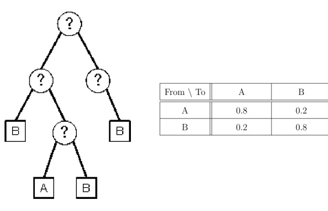
For this purpose, we use the information available from the phylogenetic trees. Let S = {s1, . . . , sn} be an input collection of n virus sequences, where n ≥ 1. Then, a phylogenetic tree(or anevolutionary tree) [8] forSis a rooted binary treeT = (V, E, root) that represents an inferred evolutionary relationship of S as shown in Fig. 1.2 (left). T has n₁ internal nodes corresponding to the virtual ancestral sequences and n₂ leaves corresponding to the real sequences inS. Each edge (x, y) means thatyis obtained from x by mutation. In addition, each leaf z is labeled by a location g(z) ∈ ∆ where the

(6)

corresponding sequence is sampled.

The organization of this thesis is as follows. In Chapter 2, we deﬁne a statistical model for generating geographic label assignments for a given phylogenetic tree. In Chapter 3, we present a Viterbi training algorithm [5] VT Tree for inferring the GTP for an input tree consisting of n=n₁+n₂ nodes, and anm×m cost matrix over a label alphabet of size m. The computation time of the algorithm is O(m²n) time by using dynamic pro- gramming [3]. In Chapter 4, we present an expectation maximization (EM) algorithm [4]

EM Tree for inferring the GTP more efficiently than VT Tree. The computation time of each iteration for inferring the GTP isO(m²n) time by using dynamic programming. In Chapter 5, we apply our algorithms to the phylogenetic tree of influenza viruses, then we estimate the GTP of influenza viruses. In Chapter 6, we conclude this thesis.

Contribution of this thesis is summarized as follows.

1. We propose a probabilistic model for label propagation on a binary tree with a given transmission probability.

2. We present two statistical inference algorithm based on Viterbi training and EM algorithm that infer the unknown transmission probability from given external labels.

By using dynamic programming, these algorithms work eﬃciently.

3. We apply the proposed algorithms to the inference of global circulation patterns of influenza viruses, and evaluate their effectiveness by experiments on artificial and real datasets.

The contents of Chapter 3 was presented in the 16th Special Interest Group on Bioin- formatics [17] and in the 20th international conference on genome informatics [16]. The contents of Chapter 4 was presented in the 80th Special Interest Group on Fundamental Problems in Artiﬁcial Intelligence [18].

(7)

Figure 1.1: A map with the geographic transmission probability (GTP) of H3N2 in- ﬂuenza virus.

(8)

From \ To A B

A 0.8 0.2

B 0.2 0.8

Figure 1.2: An example of a phylogenetic tree T (left) and an GTP table θ (right) on an alphabet ∆ ={A, B}of locations.

(9)

Chapter 2 Geographic Transmission Probability

Inference Problems for Phylogenetic Trees

2.1 Phylogenetic trees

In this chapter, we give basic deﬁnitions and notations. We deﬁne a generative model for geographic label assignments to the nodes of a given phylogenetic tree (Figure 1.2 left) as a graphical model [2, 5]. Let ∆ = {1, . . . , m} be an alphabet of m geographic labels such as Asia, North-America, South-America, Oceania, and Europe where the virus sequences are sampled. Suppose that T is a phylogenetic tree with n₁ internal nodes in V_I = {1, . . . , n₁} and n₂ leaves in V_L = {n₁ + 1, . . . , n₁ +n₂}. We denote by V(T) = V =V_I ∪V_L the set of nodes. We denote by E(T) = E the set of edges in T. Let n = n₁ +n₂ be the total size of T. For nodes x and y in T, if there is a directed edge from xto ythen we write x≤y and say thatx is the parent of y(or y is a child of x). If x≤y and x̸=y then we write x < y.

For a node x, we denote by x_L and x_R the left and right children of x, respectively.

We denote by x^′ the sibling of x such that x̸=x^′.

2.2 Geographic label assignments

Internal and external label assignments are mappings f : V_I → ∆ and g : V_L → ∆ that assign geographic labels of ∆ to internal nodes and leaves, respectively.

LetX = (x_i)ⁿ_i=1¹ andZ = (z_j)ⁿ_j=n¹⁺ⁿ²

1+1be the vectors ofn₁ internal labels andn₂external labels, respectively. Then, x_i and z_j (i ∈ V_I, j ∈ V_L) represent the labels assigned by f andg to thei-th internal node and the j-th leaf ofT, respectively. The index 0 represent

(10)

the root of T

We sometimes do not distinguish a node i from its label x_i =a∈∆ if the index i is clear from context. We introduce notations below, which will be convenient to describe our algorithms. Recall thatZ is the set of all leaves (and their label assignment). For an internal nodex and a setY ⊆(X∪Z) of nodes, we deﬁne the set of all descendants ofx byY_x ={y∈Y |x≤y}. Thus,Tx denotes the subtree ofT rooted atx, andZ_x denotes the set of all leaves below x. Furthermore, we denote the set of all leaves that are not below x by Zx = Z\Zx. Again, we identify the sets Zx and Zx with the corresponding label assignments if it is clear from context. Let X and Z be internal and external label assignments to T. For any pair (a, b) ∈ ∆² of labels, we denote by N(a, b|X, Z) the number of edges e = (x_i, x_j) in T that have the labels x_i = a and x_j = b. That is, N(a, b|X, Z) = |{(xi, xj)∈E(T)|xi =a, xj =b}|. We deﬁne N(a|X) by 1 if the label of the root is a, and 0 otherwise.

2.3 A Probabilistic model

We introduce a probabilistic model for the geographic transmission probability (GTP) inference problem, which generates internal and external label assignments from a set of input parameters called the GTP table. This model is a generalization of the hidden Markov model (HMM) [5] on sequences to a generative model on phylogenetic trees.

We deﬁne a GTP table as a set of parameters Θ = (ρ, θ) deﬁned as follows. Theroot probability (RP), the probability of the root labelx0 is given by

q(x₀) =q(x₀=a|ρ) = ρ_a, (2.1)

where a∈∆ is the label assigned to x₀ and ρ= (ρ_a)_a_∈_∆ is an m-vector with ρ_a≥0 and

∑

aρ_a = 1. The geographic transmission probability (GTP), the conditional probability for the label x_i =b of nodei and the label x_π(i)=a of its parent π(i), is given by

p(xi|x_π(i)) =p(xi=b|x_π(i)=a, θ) = θab, (2.2) where a, b∈ ∆ are the labels assigned to x_π(i), x_i, respectively, and θ = (θ_ab)_a,b_∈_∆ is an m×m-matrix with θ_ab ≥0 and ∑

bθ_ab = 1.

LetX andZ be the sets of all ofn₁ internal nodes and all ofn₂ leaves with their label assignments, respectively. Then, our probabilistic model is given by the joint probability

(11)

distribution for X and Z:

p(X, Z|Θ)

= p(Z|X,Θ)p(X|Θ) (2.3)

= q(x₀ |ρ)

n1

∏

i=1

p(x_i|x_π(i), θ)

n∏1+n2

j=n1+1

p(z_j|x_π(j), θ)

In what follows, we omit the parameter Θ such asp(X, Z) = p(Z|X)p(X) if no confusion arises.

Given a ﬁxed external label assignment Z, we have the following Markov properties on the label assignment f and g, where x, y and z are any nodes of T: (1) If x is the parent ofyand z, thenp(z|x, y) = p(z|x). (2) Ifx is the parent ofyand yis the parent of z, then p(z|x, y) = p(z|y).

2.4 The inference problem

Our ﬁnal goal is to infer an plausible GTP table Θ = (ρ, θ) from a given external label assignment Z for a phylogenetic tree T by the maximum likelihood estimation (ML-estimation) [2]. Formally, this problem is stated as follows.

The Geographic Transmission Probability Inference Problem from a Phylogenetic Tree (GTPIP):

Input: A phylogenetic tree T, an geographic label assignmentZ to the leaves of T (an external label assignment).

Task: Find the optimal GTP ˆΘ = (ρ, θ) that maximizes the likelihood of Z given Θ deﬁned byˆ

p(Z|Θ) =ˆ ∑

X

p(X, Z|Θ),ˆ (2.4)

where X is a geographic label assignment to the internal nodes of T (an internal label assignment).

In other words, this problem is equivalent to ﬁnd GTP ˆΘ by Θ = arg maxˆ

Θ p(Z|Θ)ˆ

= arg max

Θ

∑

X

p(X, Z|Θ).ˆ (2.5)

(12)

By convention, instead of the maximization of the likelihood p(Z |Θ), we use theˆ minimization of the negative log likelihood ℓ(Z), deﬁned by

ℓ(Z) =ℓ(Z|Θ) =ˆ −logp(Z|Θ).ˆ (2.6) To estimate Θ, we compute all label assignmentXfor internal nodes. Since the latent variable X can take exponentially many distinct label assignments, we cannot directly ﬁnd the optimal Θ. To solve this problem, we use the VT Tree algorithm and EM Tree algorithm in the following sections.

(13)

Chapter 3 A Viterbi Training Algorithm for Inferring Geographic Transmission Probability

In this chapter, we present the VT Tree algorithm for inferring the geographic transmission probability (GTP) Θ = (ρ, θ) by using the Viterbi training algorithm.

3.1 The Viterbi training algorithm

Our problem is to ﬁnd the optimal GTP ˆΘ = (ρ, θ) that maximizes the likelihood p(Z|Θ) ofˆ Z given ˆΘ. In other words, this problem is equivalent to ﬁnd GTP ˆΘ by

Θ = arg maxˆ

Θ p(Z|Θ)ˆ

= arg max

Θ

∑

X

p(X, Z|Θ),ˆ (3.1)

where X is a geographic label assignment for the internal nodes of T (an internal label assignment).

Since X can take exponentially many distinct values, it is hard to directly compute the optimal Θ. The Viterbi training algorithm is a greedy algorithm for computing Θ.

Given a phylogenetic treeT and the geographic label assignmentZ for its leaves as input, this algorithm ﬁrst computes the best label assignment ˆX for its internal nodes, and then computes the best parameter Θ = (ρ, θ) that maximizes the likelihood p( ˆX, Z |Θ) by using ML-estimation assuming the ﬁxed ˆX.

We give the algorithm scheme of the Viterbi training algorithm below.

The Viterbi training algorithm

Input: A phylogenetic tree T, an geographic label assignmentZ to the leaves of T (an external label assignment).

(14)

Algorithm VT Tree(∆ = {1, . . . , m}: a label alphabet, T: a phylogenetic tree, Z: a label assignment for leaves of T, Θ0= (ρ0, θ0): initial parameters):

1: (ρ, θ) = (ρ₀, θ₀)

2: M C =VT BottomUp(root, ρ, θ);

3: BL =VT TraceBack(root, M C);

4: (ρ, θ) =VT Estimate(root, BL);

5: return Θ = (ρ, θ);

Figure 3.1: The algorithm VT Tree

Step 1: Find the best ˆX from Z and Θ₀ by maximizing p( ˆX, Z | Θ₀), by the maximum likelihood method, that is, to ﬁnd

Xˆ = arg max

X p(X, Z |Θ₀) (3.2)

= arg min

X {−logp(X, Z|Θ₀)} (3.3)

= arg min

X ℓ(X, Z|Θ₀), (3.4)

where we deﬁne ℓ(X, Z|Θ₀) = −logp(X, Z|Θ₀) and call it the cost of X.

Step 2: Find the optimal ˆΘ that maximized the likelihood p( ˆX, Z|Θ) of ˆˆ X and Z given ˆΘ, that is, to ﬁnd

Θ = arg maxˆ

Θ p( ˆX, Z|Θ) (3.5)

= arg min

Θ

{−logp( ˆX, Z|Θ) }

. (3.6)

The concept of Viterbi algorithms was originally introduced in learning of hidden Markov models (HMM) [5]. In the original algorithm for HMM, the name of the Viterbi training algorithm came from the fact that Step 1 uses the Viterbi algorithm [5] for computing the most likely state sequence of an HMM on a given input sequence.

3.2 The algorithm VT Tree

Based on the algorithm scheme of the Viterbi training algorithm, we show our algorithm VT Tree in Fig. 3.1. This algorithm computes the parameter Θ from a given

(15)

external label assignmentZ as observed variables on an input phylogenetic treeT by using the Viterbi training algorithm. In theVT Tree, ﬁrstly the subprocedureVT BottomUp computes dynamic programming (DP) table M C which represent the minimum cost of Tx, by traversingT from the leaves to the root. Secondly, the subprocedureVT TraceBack computes the best label assignmentBLfor its internal nodes from tablesM C, by traversing T from the root to the leaves. Finally, the subprocedure VT Estimate computes the values of Θ = (ρ, θ) from BL.

The VT Tree consists of two parts. The ﬁrst part corresponds to Step 1 in the algorithm scheme of Viterbi training algorithm and consist of the procedures VT BottomUp and VT TraceBack. In this part, the procedures together computes the best label assignment ˆX that minimize the cost ℓ( ˆX, Z|Θ) given by

ℓ( ˆX, Z|Θ)

= −logp( ˆX, Z|Θ) (3.7)

= I_x₀ +

n1

∑

i=1

D_x_i_x_π(i)+

n∑1+n2

j=n1+1

D_z_j_x_π(j),

whereI_x =−logq(x|Θ) andD_xz =−logp(x|z,Θ). In Fig. 3.1 the procedures solve this problem by using dynamic programming (DP) [3] on an input phylogenetic tree. We see that the procedures in this part are a generalization of the Viterbi algorithm for HMMs to that for phylogenetic tree. The second part corresponds to Step 2 in the algorithm scheme of the Viterbi training algorithm and consist of the procedure VT Estimate. In this part, the procedure computes the values of Θ = (ρ, θ) that maximized the likelihood p( ˆX, Z|Θ) of ˆˆ X and Z given ˆΘ by using ML-estimation.

In the rest of this chapter, we ﬁx the label assignment Z for leaves.

3.3 The procedure VT BottomUp

In Fig.3.2, we show the subprocedure VT BottomUp for computing theM C table by traversing T in a bottom-up manner. M C[x][a] stores the minimum cost of the subtree Tx with the root label a∈∆ over all label assignments.

Now, we give a recurrence formula for computing M C as follows.

Lemma 1 (recurrence for M C) For any node x and any a∈∆, the following hold:

(16)

ProcedureVT BottomUp(x: node, (ρ, θ): parameters):

1: if x is leaf then

2: for all labela∈∆do 3: if a=g(x) then 4: M C[x][a] = 0

5: else

6: M C[x][a] =∞ 7: end if

8: end for 9: else

10: for all x’s childu do 11: VT BottomUp(u, ρ, θ);

12: end for

13: for all labela∈∆do 14: for allx’s childido

15: M C_i^a= min{D_ab+M C[xi][b]b∈∆}; 16: M C[x][a] =∑

iM C_i^a; 17: end for

18: end for 19: end if 20: return M C;

Figure 3.2: The procedure VT BottomUp

(17)

1. If x is a leaf, then

M C[x][a] =







0 if a=g(x)

∞ otherwise.

2. If x is an internal node, then M C[x][a] =∑

i

min{Dab+M C[xi][b]|b∈∆}

Proof: We suppose that each of the cost M C[x_i][b] to the subproblem used within the optimal costM[x][a] to the original problem is not optimal. By replacing the nonoptimal cost of the subproblem by the optimal one, we can get a better cost to the original problem. It is contradicting our supposition that we already had an optimal solution to the original problem. Therefore, the cost to the subproblem used within the optimal cost to the original problem is optimal and then we can compute the optimal cost of the original problem M C[x][a] by the recurrence equation as above.

By the above recurrence, we have the following lemma.

Lemma 2 The procedureVT BottomUpin Fig. 3.2 correctly computes the tableM C[x][a]

for any node x and labela∈∆for a phylogenetic tree T and the leaf label assignmentZ. Proof: In Fig. 3.2, for a node x, the procedure VT BottomUp computes the table M C[x][a] correctly for any labela from line 2 to line 8 (ifx is a leaf) and from line 13 to line 18 (if x is an internal node) by Lemma 1. And then, since the procedure visits all nodes from leaves to the root from line 10 to line 12, the procedure correctly computes the table M C[x][a] for any node x and labela.

Lemma 3 The procedure VT BottomUp in Fig. 3.2 runs in O(m²n) time on T.

Proof: Firstly, for a labela, the procedure VT BottomUpin Fig. 3.2 computesM C_i^ain O(m) time at line 15. Then, the procedure iteratively computes M C[x][a] for a node x for each label a, in O(m²) time from line 13 to line 18. Finally, the procedure iteratively visits all nodes x and computesM C[x][a]. Therefore, the procedure VT BottomUp runs in O(m²n) time.

(18)

ProcedureVT TraceBack(x: node, M C):

1: if x is leaf then 2: BL[x] :=g(x);

3: else

4: BL[x] =argmin_a{M C[x][a]|a∈∆} 5: for all x’s childu do

6: VT TraceBack(u, M C);

7: end if 8: return BL;

Figure 3.3: The procedure VT TraceBack

3.4 The procedure VT TraceBack

In Fig.3.3, we show the subprocedure VT TraceBack for computing the best label assignment BL[x] for node xby traversing T in a top-down manner.

Now, we give a formula for computing BL as follows.

Lemma 4 (formula for BL) For any node x and any a∈∆, the following hold:

1. If x is a leaf then BL[x] =g(x).

2. If x is an internal node, then

BL[x] = arg min

a {M C[x][a]|a∈∆}.

Lemma 5 The procedure VT TraceBack in Fig. 3.3 correctly computes the table BL[x]

for any node x and label a∈∆ for a phylogenetic tree T and the table M C.

Proof: In Fig. 3.3, for a nodex, the procedureVT TraceBackcomputes the tableBL[x]

correctly at line 2 (if x is a leaf) and at line 4 (if x is an internal node) by Lemma 4.

Then, since the procedure visits all nodes from the root to leaves from line 5 to line 6, the procedure correctly computes the table BL[x] for any node x.

Lemma 6 The procedure VT TraceBack in Fig. 3.3 runs in O(mn) time on T.

(19)

Procedure VT Estimate(x: node, BL):

1: For every a, b∈∆, compute θ_ab by:

θab = A[a, b]

∑

b^′∈∆(A[a, b^′]);

2: For every a∈∆, computeρ_a by:

ρ_a = R[a]

∑

a^′∈∆(R[a^′]);

3: return (ρ, θ);

Figure 3.4: The procedure VT Estimate

Proof: In Fig. 3.3, for each nodex, the procedureVT TraceBackﬁnd the label a which minimize the costBL[x] inO(m) time. Then, the procedure iteratively visits all nodesx and computes the tables BL[x]. Therefore, the procedure VT TraceBack runs in O(mn) time.

3.5 The procedure VT Estimate

In this section, we present the procedure VT Estimate which ﬁnd the optimal ˆΘ = (ρ, θ) that maximized the likelihood p( ˆX, Z |Θ) of ˆˆ X and Z given ˆΘ by using ML estimation.

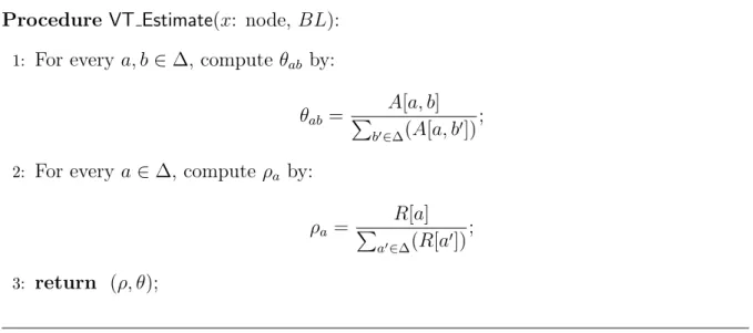
Now, we define an m×m matrix A[·][·], called the edge count table and an m-vector R[·], called the root count table as follows. For every pairs of labels a, b∈∆, we define the value A[a][b] which is defined by the number of edges e = (x_i, x_j) having the labels x_i = a and x_j = b ∈ ∆. We can compute the A[a][b] for all pairs of labels a, b ∈ ∆ by directly counting the number of edges, from the best label assignment BL for internal nodes. For any labels a ∈ ∆, we define the value R[a] which is defined by the number of the root x₀ having the labels x₀ = a. We can compute the R[a] from the best label assignment BL for root node.

In Fig.3.4, we show the procedure VT Estimate for updating the values of Θ = (ρ, θ) from these vectors A and R by using ML estimation.

(20)

Lemma 7 The procedure VT Estimate in Fig. 3.4 runs in O(m²) time.

Proof: In Fig. 3.4, the procedure VT Estimate computes the parameter θ_ab for each label a, b∈∆ in O(m²) time at line 1. Therefore, the result follows.

Theorem 8 The algorithmVT Treeof Fig. 3.1 takes O(m²n) time andO(mn)space on T, where m =|∆|is the size of a label alphabet and n =O(||T ||) is the number of leaves.

Proof: Since each node x has the m-vector M C, VT Tree takes O(mn) space. Then, by Lemma 3, Lemma 6, and Lemma 7, VT Tree takes O(m²n) time.

(21)

Chapter 4 An EM Algorithm for Inferring Geographic Transmission Probability

In this chapter, we present the EM Treealgorithm for inferring the geographic transmission probability (GTP) Θ = (ρ, θ) by using the EM algorithm.

4.1 The EM algorithm

Our problem is to ﬁnd the optimal GTP ˆΘ = (ρ, θ) that maximizes the likelihood p(Z|Θ) ofˆ Z given ˆΘ as described in section 2.4. In other words, this problem is equivalent to ﬁnd GTP ˆΘ by

Θ = arg maxˆ

Θ p(Z|Θ)ˆ

= arg max

Θ

∑

X

p(X, Z|Θ),ˆ (4.1)

where X is a geographic label assignment to the internal nodes of T (an internal label assignment).

Since X can take exponentially many distinct values, it is hard to directly compute the optimal Θ. To solve this problem, we propose our algorithm EM Tree based on a general algorithmic scheme forexpectation maximization(EM) algorithms (e.g., [4, 5, 7]).

The learning parameters to the algorithm are an initial model parameter Θ₀ = (ρ₀, θ₀) for GTP and a threshold ε > 0 for convergence. Given a phylogenetic tree T and a geographic label assignmentZ for its leaves as inputs, starting from the initial parameter Θ₀ = (ρ₀, θ₀), the algorithm EM Tree iteratively computes the improved parameter Θ = (ρ, θ) that locally maximizes the likelihood p(Z |Θ) among all possible Θ by using ML- estimation.

(22)

We give the algorithm scheme of the EM algorithm below.

The Expectation Maximization algorithm

Input: A phylogenetic tree T, a geographic label assignment Z to the leaves of T (an external label assignment), an initial model parameter Θ₀, a threshold for convergence ε.

Step 1: Initialize the GTP Θ₀ = (ρ₀, θ₀).

Step 2: Main loop. Repeat the following steps while ℓ_last−ℓ > ε, where ℓ is the negative log likelihood−logp(X|Θ) from the parameter Θ andℓ_last is the negative log likelihood of the last repetition:

Step 2.1: Expectation step. For every edge (x_i, x_j) of treeT, ﬁnd the expected value of the number of edges N(a, b|X, Z) having the labels xi = a and x_j =b∈∆, that is, to ﬁnd

A[a][b] = E_X^Θ[N(a, b|X, Z)|Θ0] (4.2)

= ∑

x∈X∪Z:x̸=root

p(π(x)=a, x=b|Z,Θ0), (4.3) for any labels a, b ∈ ∆, and ﬁnd the expected value of the number of root N(a|Z) having the labels x₀ =a, that is, to ﬁnd

R[a] = E_X^Θ[N(a|Z)|Θ₀] (4.4)

= p(x=a|Z,Θ₀), (4.5)

for any labelsa∈∆.

Step 2.2: Maximization step. Find the optimal ˆΘ that maximized the likelihood p(Z|Θ) ofˆ Z given ˆΘ, that is, to ﬁnd

Θ = arg maxˆ

Θ p(Z |Θ) (4.6)

= arg max

Θ

∑

X

p(X, Z|Θ). (4.7)

Lemma 9 For any labels a, b∈∆,

E_X^Θ[N(a, b|X, Z)|Θ0] = ∑

x∈X∪Z:x̸=root

p(π(x)=a, x=b|Z,Θ0).

(23)

Proof:

E_X^Θ[N(a, b|X, Z)|Θ₀]

= E_X^Θ

[ ∑

x∈X∪Z:x̸=root

δ(a, b|x, X) ]

(by the deﬁnition of N(a, b|X, Z).)

= ∑

x∈X∪Z:x̸=root

E_X^Θ[δ(a, b|x, X)] (by linearity of expectation in Lemma 29.)

= ∑

x∈X∪Z:x̸=root

∑

X

p(π(x)=a, x=b|X, Z,Θ₀)·δ(a, b|x, X) (by the deﬁnition of expectation in Deﬁnition 11.)

= ∑

x∈X∪Z:x̸=root

∑

X

p(π(x)=a, x=b|X, Z,Θ₀) (by the deﬁnition ofδ below.)

= ∑

x∈X∪Z:x̸=root

p(π(x) = a, x=b|Z,Θ₀) (by marginalization over X.), where

δ(a, b|x, X) =







1 π(x)=a, x=b, 0 otherwise.

The concept of EM algorithms was originally introduced by Dempster, Laird, and Ru- bin [4]. The name of the EM algorithm came from the fact that the algorithm alternately executes the expectation step and the maximization step.

4.2 The algorithm EM Tree

Based on the algorithm scheme of the EM algorithm, we show in Fig. 4.1, our algorithm EM Tree. This algorithm computes the parameter Θ from a given external label assignmentZ as observed variables on an input phylogenetic treeT by using the EM algorithm with latent variables X. In the main loop of EM Tree, ﬁrstly, the subprocedures EM BottomUpandEM TopDowncomputem-vectorsP BU[x][·] andT D[x][·]∈[0,1]^m for every node x ofT, by traversingT from the leaves to the root and from the root to the leaves respectively. Secondly, the subprocedure EM ExpectedCount computes the edge count table A[·][·] and the root count table R[·]. Finally, the subprocedure EM Estimate updates the values of Θ = (ρ, θ) from these tables A[·][·] and R[·]. The main loop is

(24)

Algorithm EM Tree(∆ = {1, . . . , m}: a label alphabet, T: a phylogenetic tree, Z: a label assignment for leaves of T, Θ0 = (ρ0, θ0): initial parameters, ε: threshold for convergence):

1: (ρ, θ) = (ρ₀, θ₀);

2: while (ℓ_last−ℓ > ε) do

3: ℓ_last =ℓ;

4: P BU =EM BottomUp(root, ρ, θ);

5: T D=EM TopDown(root, ρ, θ);

6: (R, A) =EM ExpectedCount(P BU, T D, ρ, θ);

7: (ρ, θ, ℓ) = EM Estimate(R, A);

8: end while

9: return Θ = (ρ, θ);

Figure 4.1: The algorithm EM Tree

iterated until the change in log likelihood ℓ(Z) =ℓ(Z |Θ) is less than a given threshold ε >0 or the maximum number of iterations is exceeded.

The EM Tree consists of two steps. The ﬁrst step called Expectation step (E-step) corresponds to Step 2.1 in the algorithm scheme of EM algorithm and consist of the procedures EM BottomUp, EM TopDown, and EM ExpectedCount. In this step, the procedures together computes the expected value of the number of edges A[a][b] having the labels x_i = a and x_j = b ∈ ∆, and expected value of the number of the root R[a] hav- ing the labels x₀ = a. In Fig. 4.1 the procedures solve this problem by using dynamic programming (DP) [3] on an input phylogenetic tree T. We see that the procedure EM BottomUp and EM TopDown in this step are a generalization of the forward algorithm and the backward algorithm [5] respectively for HMMs to that for phylogenetic tree. The second step called Maximization step (M-step) corresponds to Step 2.2 in the algorithm scheme of the EM algorithm and consist of the procedure EM Estimate. In this step, the procedure computes the values of Θ = (ρ, θ) that maximized the likelihood p(Z|Θ) of Z given Θ by using ML-estimation.

In the rest of this chapter, we ﬁx the label assignment Z for leaves.

(25)

Procedure EM BottomUp(x: node, (ρ, θ): parameter):

1: if x is leaf then

2: for each label a∈∆do P BU[x][a] =θ_ag(x);

3: else

4: EM BottomUp(x_L, ρ, θ);

5: EM BottomUp(x_R, ρ, θ);

6: for each label a∈∆do P BU[x][a] =

∑

b∈∆{P BU[x_L][b]·P BU[x_R][b]·θ_ab};

7: end if

8: return P BU;

Figure 4.2: The procedure EM BottomUp

4.3 The procedure EM BottomUp

In Fig. 4.2, we show the recursive procedureEM BottomUpfor computing theP BU table by traversing T in a bottom-up manner.

For each node x in T, we deﬁne the following tables with respect to the subtree Tx =X_x∪Z_x of T rooted atx, where a is any label:

• The valueBU[x][a] is deﬁned by the probability BU[x][a] =p(Zx|x=a) = ∑

Xx:x=a

p(Zx, X). (4.8)

• The valueP BU[x][a] is deﬁned by the probability P BU[x][a] =p(Z_x|π(x)=a) = ∑

Xx

p(Z_x, X), (4.9)

where π(x) is the parent of x.

The next lemma says that BU[x][a] and P BU[x][a] are interchangeable each other.

Lemma 10 For every node x, the following equation hold:

BU[x][a] =P BU[x_L][a]·P BU[x_R][a].

(26)

Proof: By deﬁnition, we have BU[x][a] = p(Z_x |x = a). Since x has exactly two children x_L and x_R, we can split Z_x asZ_x =Z_x_L∪Z_x_R. Thus, we have p(Z_x|x =a) = p(Z_x_L|x= a)·p(Z_x_R |x =a). Then, we can show that p(Z_x_L|x =a) = p(Z_y |π(y) = a) = P BU[y][a] = P BU[x_L][a], where we put y = x_L and π(y) = x. Similarly, we can also show that p(Z_x_L | x = a) = P BU[x_L][a]. Combining the above discussion, BU[x][a] =P BU[x_L][a]·P BU[x_R][a].

Lemma 11 For every node x, the following equation hold:

P BU[x][a] =∑

b∈∆

BU[x][b]·θ_ab. Proof: We show the following.

P BU[x][a]

= p(Z_x|π(x) =a) (by the deﬁnition ofP BU.)

= ∑

b∈∆

p(Z_x|x=b)·p(x=b|π(x) =a) (by Lemma 27.)

= ∑

b∈∆

BU[x][b]·θ_ab (by the deﬁnition of BU[x][a] andθ_ab.).

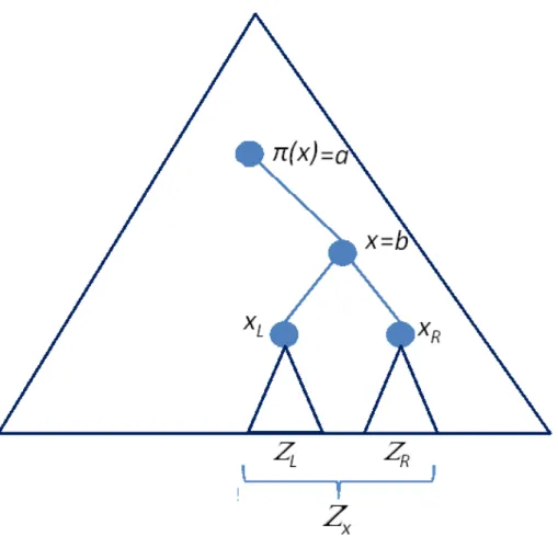
Now, we give a recurrence formula for computing P BU as follows (Fig. 4.3).

Lemma 12 (recurrence for P BU) For any node x and any labela∈∆, the following hold:

1. If x is a leaf then P BU[x][a] =θ_ag(x). 2. If x is an internal node, then

P BU[x][a]

= ∑

b∈∆

{P BU[x_L][b]·P BU[x_R][b]·θ_ab}.

(27)

Figure 4.3: Computation of the PBU table on the subtreeTX

(28)

Proof: We show the following.

P BU[x][a]

= p(Z_x|π(x) =a) (by the deﬁnition ofP BU.)

= ∑

b∈∆

{p(Z_x|x=b)·p(x=b|π(x) =a)} (by Lemma 27.)

= ∑

b∈∆

{p(Z_x_L|x=b)·p(Z_x_R |x=b)·p(x=b|π(x) =a)} (becauseZ_x=Z_x_L∪Z_x_R.)

= ∑

b∈∆

{P BU[x_L][b]·P BU[x_R][b]·θ_ab} (by the deﬁnition of P BU and θ_ab.).

Lemma 13 The procedureEM BottomUpin Fig. 4.2 correctly computes the tableP BU[x][a]

for any node x and labela∈∆for a phylogenetic tree T and the leaf label assignmentZ. Proof: For a node x, the procedure EM BottomUp in Fig. 4.2 computes the table P BU[x][a] correctly for any nodexand any label a at line 2 (if xis a leaf) and line 6 (if xis an internal node) by Lemma 12. Then, since the procedure visits all nodes from leaves to the root from line 4 to line 5, the procedure correctly computes the table P BU[x][a]

for any node xand label a.

Lemma 14 The procedure EM BottomUp in Fig. 4.2 runs in O(m²n) time on T. Proof: In Fig. 4.2, the procedureEM BottomUpcomputes the tableP BU[x][a] for each label a in O(m²) time from line 6 to line 7. Then, the procedure iteratively visits all nodes x and computes the table P BU. Therefore, the procedure EM BottomUp runs in O(m²n) time.

4.4 The procedure EM TopDown

In Fig. 4.4, we show the recursive procedure EM TopDown for computing the T D table by traversing T in a top-down manner.

For each node x in T, we deﬁne the following table with respect to the subgraph Tx = T \Tx that is obtained from T = X ∪Z by removing the subtree Tx = X_x∪Z_x

(29)

Procedure EM TopDown(x: node, (ρ, θ): parameters):

1: if x is the root x₀ then

2: for each label a∈∆do T D[x][a] =ρ_a;

3: else

4: for each label a∈∆do T D[x][a] =

∑

b∈∆{P BU[x^′][b]·θ_ba·T D[π(x)][b]};

5: end if

6: EM TopDown(x_L, ρ, θ);

7: EM TopDown(x_R, ρ, θ);

8: return T D;

Figure 4.4: The procedureEM TopDown

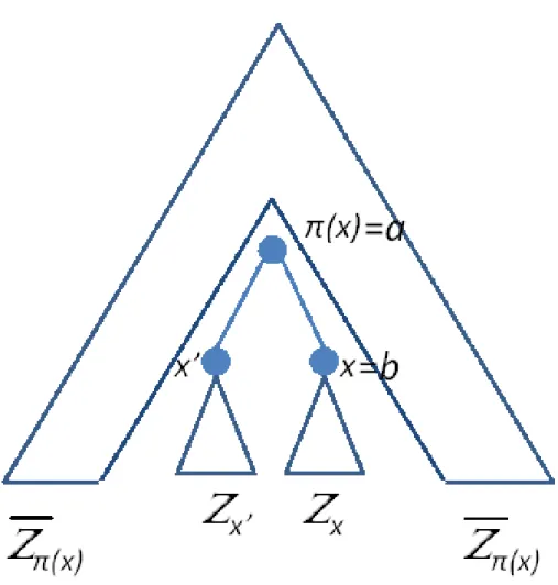
rooted at x. See Fig. 4.5 for an example of Tx. Then, for any label a, the value T D[x][a]

is deﬁned by the probability

T D[x][a] =p(Z_x, x=a). (4.10) Now, we give a recurrence formula for computing T D as follows (Fig. 4.5).

Lemma 15 (recurrence for T D) For any node x and any a∈∆, the following hold:

1. If x is the root x₀ then T D[x₀][a] =ρ_a. 2. If x is an internal node but the root, then

T D[x][a]

= ∑

b∈∆

{P BU[x^′][b]·T D[π(x)][b]·θba},

where x^′ is the sibling of x such that x̸=x^′.

(30)

Figure 4.5: Computation of the TD table on the anti-subtree Tx

(31)

Proof: We show the following.

T D[x][a] = p(Z_x, x=a) (by the deﬁnition of TD.)

= ∑

π(x)=b

p(Z_x, x=a, π(x) =b) (by marginalization.)

= ∑

π(x)=b

p(Z_x′, Z_π(x), x=a, π(x) = b) (because Z_x =Z_x′ ∪Z_π(x).)

= ∑

π(x)=b

p(Z_x′, x=a|Z_π(x), π(x) = b)·p(Z_π(x), π(x) = b)

(by the deﬁnition of the conditional probability in Deﬁnition 4.)

= ∑

π(x)=b

p(Z_x′, x=a|π(x) =b)·T D[π(x)][b]

(by Markov property and the deﬁnition of T D.)

= ∑

π(x)=b

p(Z_x′ |π(x) = b)·p(x=a|π(x) =b)·T D[π(x)][b] (by Markov property.)

= ∑

π(x)=b

P BU[x^′][b]·T D[π(x)][b]·θba (by the deﬁnition ofP BU and θab.).

Lemma 16 The procedureEM TopDownin Fig. 4.4 correctly computes the tableT D[x][a]

for any node x and labela∈∆for a phylogenetic tree T and the leaf label assignmentZ. Proof: In Fig. 4.4, for a nodex, the procedureEM TopDowncomputes the tableT D[x][a]

correctly for any label a at line 2 (if x is a leaf) and line 4 (if x is an internal node) by Lemma 15. Then, since the procedure visits all nodes from the root to leaves from line 6 to line 7, the procedure correctly computes the table T D[x][a] for any node x and label a.

Lemma 17 The procedure EM TopDown in Fig. 4.4 runs in O(m²n) time on T.

Proof: In Fig. 4.4, the procedure EM TopDown computes the table T D[x][a] for each label a in O(m²) time from line 4 to line 5. Then, the procedure iteratively visits all nodes x and computes the table T D. Therefore, the procedure EM TopDown runs in O(m²n) time.

(32)

Procedure EM ExpectedCount((ρ, θ): parameters, P BU, T D):

1: for each label a∈∆ do

2: R[a] =p(x=a|Z).

3: end for

4: for each label a∈∆ do

5: for each label b∈∆ do

6: A[a][b] =∑

x∈X∪Z:x̸=root{p(π(x)=a, x=b|Z)};

7: end for

8: end for

9: return (R, A);

Figure 4.6: The procedure EM ExpectedCount

4.5 The procedure EM ExpectedCount

In Fig. 4.6, we show the procedure EM ExpectedCount for computing the tableA[·][·] and table E[·] which represent the expected value of the number of edge count and the expected value of the number of root count respectively.

First, we give the likelihood of the whole data Z in terms of the tables P BU. Let x_0L and x_0R be the left and right children of the root x₀.

Lemma 18 For an input leaf label assignment Z, we have:

p(Z) =∑

a

P BU[x0L][a]·P BU[x0R][a]·ρa. (4.11) Proof: SinceZ =Z_x₀, we havep(Z) =∑

ap(Z|x₀=a)·p(x₀=a) =∑

aBU[root][a]·ρ_a. From Lemma 10, the result follows.

From the above lemma, we have the posterior probability of x=a as follows.

Lemma 19 For any internal nodex, we have the following joint probability, wherea ∈∆ is any label:

p(x=a|Z) = BU[x][a]·T D[x][a]/ p(Z). (4.12)

(33)

Proof: By partitioning the whole treeT intoTx andTx, we havep(Z, x=a) =p(Z_x|x=

a)·p(Z_x, x=a). Since BU[x][a] =p(Z_x|x=a) andT D[x][a] =p(Z_x, x=a) by deﬁnitions, we have p(Z, x=a) = BU[x][a]·T D[x][a], and thus, the lemma follows.

Finally, we have the edge probability (Fig. 4.7).

Lemma 20 (edge probability) For any internal nodex, we have the conditional prob- ability p(π(x)=a, x=b|Z) as follows:

• If x is an internal node, then

p(π(x)=a, x=b|Z)

= θ_ab·T D[π(x)][a]·P BU[x^′][a]· P BU[x_L][b]·P BU[x_R][b]/ p(Z).

• If x is a leaf, then

p(π(x)=a, x=b|Z)

= θ_ab·T D[π(x)][a]·P BU[x^′][a]/ p(Z), where a, b∈∆ are any labels.

(34)

Figure 4.7: Explanation of Lemma 20

(35)

Proof: If x is an internal node, then p(π(x)=a, x=b, Z)

= p(π(x)=a, x=b, Z_π(x), Z_π(x)) (because Z=Z_π(x)∪Z_π(x).)

= p(x=b, Z_π(x)|π(x)=a, Z_π(x))·p(π(x)=a, Z_π(x))

= p(x=b, Z_π(x)|π(x)=a, Z_π(x))·T D[π(x)][a] (by the deﬁnition of T D.)

= p(x=b, Z_π(x)|π(x)=a)·T D[π(x)][a] (by Markov property.)

= p(x=b, Zx, Zx^′ |π(x)=a)·T D[π(x)][a] (because Z_π(x)=Zx∪Zx^′.) (4.13)

= p(Zx|x=b, Zx^′, π(x)=a)·p(x=b, Zx^′ |π(x)=a)·T D[π(x)][a]

= p(Zx|x=b)·p(x=b, Zx^′|π(x)=a)·T D[π(x)][a] (by Markov property.)

= p(Zx|x=b)·p(Zx^′ |x=b, π(x)=a)·p(x=b|π(x)=a)·T D[π(x)][a]

= p(Zx|x=b)·p(Zx^′ |π(x)=a)·p(x=b|π(x)=a)·T D[π(x)][a] (by Markov property.)

= p(x=b|π(x)=a)·BU[x][a]·P BU[x^′][a]·T D[π(x)][a] (by the deﬁnition ofBU and P BU.)

= θab·P BU[xL][b]·P BU[xR][b]·P BU[x^′][a]·T D[π(x)][a] (by Lemma 10.).

Therefore, we have

p(π(x)=a, x=b|Z) =θ_ab·P BU[x_L][b]·P BU[x_R][b]·P BU[x^′][a]·T D[π(x)][a]/p(Z).

If x is a leaf, in Equation 4.13, Z_x =x. Hence, we have

p(π(x)=a, x=b, Z) = p(x=b, x, Zx^′ |π(x)=a)·T D[π(x)][a] (by Equation 4.13.)

= p(x=b, Zx^′ |π(x)=a)·T D[π(x)][a] (by derivation.)

= p(x=b|π(x)=a)·p(Zx^′|π(x)=a)·T D[π(x)][a] (by Markov property.)

= θab·P BU[x^′][a]·T D[π(x)][a] (by the deﬁnition of P BU and θab.).

Therefore, we have

p(π(x)=a, x=b|Z) =θ_ab·P BU[x^′][a]·T D[π(x)][a]/p(Z).

(36)

Now, we define an m×m matrix A[·][·], called the expected edge count table and an m-vector R[·], called the expected root count table as follows. For every pairs of labels a, b ∈ ∆, we define the value A[a][b] which is defined by the expected number of edges e= (x_i, x_j) having the labels x_i =a and x_j =b ∈∆ by

A[a][b] = ∑

x∈X∪Z:x̸=root

p(π(x)=a, x=b|Z). (4.14)

Lemma 21 For any labels a, b∈∆, the edge count table A[a][b] is given by:

A[a][b] = ∑

x:leaf

{θ_ab·T D(π(x), a)·P BU[x][b]· P BU[x^′][a]/ p(Z)}

+ ∑

x:internal

{θab·T D[π(x)][a]·P BU[x^′][a]· P BU[x_L][b]·P BU[x_R][b]/ p(Z)}. Proof: Immediately from Lemma 20.

For any labels a ∈ ∆, we deﬁne the value R[a] which is deﬁned by the expected number of the root x₀ having the labels x₀ =a by

R[a] =p(x=a|Z). (4.15)

Lemma 22 For any labels a∈∆, the root count table R[a] is given by:

R[a] =ρ_a·P BU[x_0L][a]·P BU[x_0R][a]/ p(Z). (4.16) Proof: Clearly, p(Z, x₀=a) =p(Z_x₀ |x₀=a)·ρ_a. Since p(Z_x₀ |x₀=a) = BU[x₀][a] = P BU[x_0L][a]·P BU[x_0R][a] from Lemma 10, the result follows.

Lemma 23 The procedure EM ExpectedCount in Fig. 4.6 correctly computes the table R[a] for any label a∈∆ and the table A[a][b] for any label a, b∈∆.

Lemma 24 The procedure EM ExpectedCount in Fig. 4.6 runs in O(m²n) time on T. Proof: From Lemma 21, to compute a table A[a][b], the procedure EM ExpectedCount visits all nodesx∈X∪Z :x̸=root. Therefore, the procedure computes the tableA[a][b]

for any label a, b ∈ ∆ in O(m²n) time from line 4 to line 8. As a result, the procedure EM ExpectedCount runs in O(m²n) time.

(37)

Procedure EM Estimate(R, A):

1: For every a, b∈∆, compute θ_ab by:

θab = A[a, b]

∑

b^′∈∆(A[a, b^′]);

2: For every a∈∆, computeρ_a by:

ρ_a = R[a]

∑

a^′∈∆(R[a^′]);

3: Compute the negative log likelihood ℓ(Z) by:

ℓ =ℓ(Z) =−logp(Z |ρ, θ);

4: return (ρ, θ, ℓ);

Figure 4.8: The procedureEM Estimate

4.6 The procedure EM Estimate

In Fig. 4.8, we show the procedureEM Estimate for updating the values of Θ = (ρ, θ) that maximized the likelihood p(X, Z |Θ) from these tables R and A by using ML estimation of multinomial distributions.

The procedureEM Estimatein Fig. 4.8 computes the estimation of the root probability ρ, the transmission probability θ, and the negative log likelihood ℓ from tables R and A using a given pseudo countα >0.

Lemma 25 The procedure EM Estimate in Fig. 4.8 runs in O(m²) time.

Proof: In Fig. 4.8, the procedure EM Estimate computes the parameter θ_ab for each label a, b∈∆ in O(m²) time at line 1. Therefore, the result follows.

We have the time complexity of the update of parameter Θ = (ρ, θ) by our EM algorithm.

Theorem 26 Each iteration of the while-loop in the algorithmEM Tree of Fig. 4.1 takes O(m²n) time and O(mn) space on T, where m =|∆| is the size of a label alphabet and n =O(||T ||) is the number of leaves.

(38)

Proof: Since each nodexhas the m-vectorP BU andT D,EM TreetakesO(mn) space.

Then, by Lemma 14, Lemma 17, and Lemma 25, EM Tree takes O(m²n) time.

4.7 Extension with prior distribution

We can extend our probabilistic model for GTP by introducing prior distribution for parameter Θ = (ρ, θ) in Bayesian framework [2] as follows. We model the priors for θ and ρby Dirichlet distributionsDir(· |α₀) and Dir(· |β₀) with hyper-parametersα₀ and β0. Then, the joint probability distribution for X, Z, and Θ is given by:

p(X, Z,Θ|α₀, β₀)

= p(Z|X,Θ)p(X|Θ)q(Θ|α₀, β₀), (4.17) where

q(Θ|α₀, β₀) = q(θ|α₀)q(ρ|β₀) (4.18)

θ|α₀ ∼ Dir(· |α₀) (4.19)

ρ|β₀ ∼ Dir(· |β₀). (4.20)

In this case, our problem is the maximum a posteriori estimation (MAP-estimation) of the parameter Θ = (ρ, θ) to ﬁnd Θ that maximizes a posteriori probability of Θ:

p(Θ|Z, α₀, β₀)

∝ p(Z,Θ|α₀, β₀)

= p(Z|Θ) p(Θ|α₀, β₀)

∝ logp(Z|Θ) + logp(Θ|α₀, β₀). (4.21) To ﬁnd the parameters Θ = (ρ, θ) that maximizes Equation (4.21), we use the MAP solution for multinomial distribution with Dirichlet prior ([7]). For this purpose, we modify the procedure EM Estimate of Fig. 4.8 by replacing the code from line 3 to line 4 with the code in Fig. 4.9 using a pseudo count α as a hyper-parameter.

In the modiﬁed EM algorithm, the Expectation step is identical as the original version of EM Tree. In the Maximization step, the above code tries to maximize

E_Θ′[logp(Θ|Z, X)|Z] (4.22)

∝ E_Θ′[logp(Z, X|Θ)|Z] + logp(Θ|α₀, β₀),