Crete Island, Greece, 5–10 June 2016
FLUID ANALYSIS
USING FICTITIOUS DOMAIN FINITE ELEMENT METHOD
Y. Terakado
1, and T. Kurahashi
21
Graduate school of Nagaoka University of Technology 1603-1 Kamitomioka, Nagaoka, Niigata, Japan
e-mail: [email protected]
2
Department of Mechanical Engineering, Nagaoka University of Technology 1603-1 Kamitomioka, Nagaoka, Niigata, Japan
[email protected]
Keywords: Fictitious domain method, Finite element method, Lagrange multiplier method, Incompressible viscose flow, Background domain, Foreground domain.
Abstract. When the fluid analysis is carried out in the case that there is a moving object in the flow field, the mesh regeneration method is applied due to the Adaptive mesh refinement method. In addition, the Shear-Slip mesh update method is employed in case of rotating body problems. On the other hand, a method using the flow domain overlapped with the moving object is also proposed. In the finite difference method, a foreground grid is represented by moving object, and a main-grid is used for flow field calculation. The Overset-grid is applied to the fluid analysis to reflect the foreground grid to main-grid by the least-squares method.
Furthermore, the Immersed boundary method based on the finite volume method is also em-
ployed. In the finite element analysis, the fictitious domain method is often adopted for the
moving body problems. In this method, the computational domain is divided into foreground
domain and back-ground domain. In addition, the formulation is carried out based on the La-
grange multiplier method, and is applied to consider the velocity condition in the foreground
domain. The finite element fluid analysis is carried out to reflect the physical quantity of the
foreground domain to back-ground domain. Physical quantities at any points of the fore-
ground domain can be obtained from the physical quantities at each node by interpolation
method. In this study, the flow field analysis using the fictitious domain finite element method
is carried out.
1 INTRODUCTION
When fluid analysis is carried out, the finite element method (FEM) is often employed, and is widely used as one of the most common analysis techniques. However, if the object moves in the flow field, it is necessary to re-generate the element mesh for the calculation each time, there is a problem that the computational cost increases. On the other hand, the fictitious do- main method [1, 2] is employed as an analysis technique using two element areas within the object and the flow field in the background. Therefore, it is not necessary to re-generate the background mesh even if the object moves. This approach formulated based on the method of Lagrange multiplier [3, 4], representing the background and foreground meshes. Analysis of the flow field to perform a physical quantity of the foreground mesh is reflected to the back- ground mesh by using the interpolation method. This study is to verify the numerical analysis of incompressible viscous fluid with a fictitious domain method.
Figure 1: Example of finite element mesh in the fictitious domain method.
2 DISCRETIZATION OF THE GOVERNING EQUATIONS 2.1 Governing equation
The Navier-Stokes and the continuity equations are used to represent flow behavior and are written as Equations (1) and (2):
i j ji
j i ij i j
i
u u P u u f
u
1 1
, , , ,
,
(1)
,i
0
u
i(2)
where V
i, P, Re, and f
idenote the flow velocity, pressure, Reynolds number, and body force per unit volume, respectively.
2.2 Discretization of the governing equation
As a method to solve the equation, the splitting method is applied. In this approach, it is possible to solve the equation by separating the pressure and velocity.
First, to get the solution of the pressure field, we derive the pressure Poisson equation. Per- forming discretization in the time direction using the Euler method to Equation (1), to give Equation (3).
j inn i j n
j i n
i n
j i n j n i n
i
u u P u u f
t u u
1 1
, , , 1 , ,
1
(3)
Since the flow velocity is interpolated using triangular primary element, the term of the third order differentiation and differential term of constant value are vanished. The equation which was rewritten to Poisson equation of pressure is shown in Equation (4).
i n
j i n j n
i i n
ii
u u u
P t
, , ,
1 ,
1 (4)
When it is assumed that the weighting function P* relates to a pressure P, the weighted resid- ual equation is as shown in Equation (5).
d n P P
d n u P u d
u P u d u t P d
P P
i n e i
i n
j e i n j n
j e i i n j n
i e i n
e i i 1
*
,
* ,
* , ,
* 1
,
* ,
1
(5)
Next, if the Crank-Nicolson method is applied to the momentum equation, Equation (6) is obtained.
n i j
n i j n
j i n
i n
j i n j n i n
i
u u P u u f
t u u
1 1
, 2 1 , 2 1 , 1
, 2
1 , 1
(6) Multiplying the weighting function u
i*on the flow velocity for both sides of Equation (6), integrating over the domain Ω
e, and introducing the term of the Lagrange multiplier λ
i[3, 4], Equation (7) is consequently obtained.
e
n i i
w n i e i
j n
i j n
j i n
i n
j i n j n
i n i i
d t f u
d u d
u u t t P
u tu u
u u
*
1
* ,
2 1 , 2 1 , 1
, 2
1 , 1
*
1
(7)
In addition, by introducing an interpolation function by the triangular and the bubble func- tion elements, Equations (8) and (9) are finally obtained.
yx yy
ny nn x xy xx n
y y n x x n
yy
xx
C p t S v S v D D v D D v b
C
11
(8)
n
y x y x n
y x
n
y x y x yy
t yx t
xy t xx n t
y x y x
n
y x y x
y x
T y yy
t yx t
T x xy t xx n t
y x y x
t t t
t
f f t t
0 0
p A
p A
r r v v
0 0 0 0
0 0 0 0
0 0 H H
0 0 H H
r r v v
0 0 0 0
0 0 0 0
0 0 M 0
0 0 0 M
r r v v
0 0 B
0
0 0 0
B
B 0 H H
0 B H H
r r v v
0 0 0 0
0 0 0 0
0 0 M 0
0 0 0 M
1
2 2
2 2
1
2 2
2 2
1
(9)
The matrices and vectors in the finite element equation for the pressure Poisson equation and the momentum equation are shown in Equations (10) and (11), respectively.
y
y y y y
TT x x x x x
T
y n y n
y y n y n
y x n
e x y
n x n
y x n y n
x x n x
e
T y B y T B y e yy
T x B x T B y yx
e
T y B y T B x e xy
T x B x T B x xx
e T
y B e y
T x B x
e T
y y e yy
T x x xx
V V V V V
V V V
P P P
d n P V V V V n P V V V V
d d
d d
d d
d d
4 3 2 1 4
3 2 1
3 2 1
1 , , ,
1 , , ,
, ,
, ,
, ,
, ,
, ,
, , ,
,
, ~
~ , , ,
,
v v
p
N b
N v N N D
N v N N D
N v N N D
N v N N D
NN S
NN S
N N C
N N C
(10)
a f a
f
N T t
N T t
a r
a r
v v
p
a a
a a
B
a a
a a
B
N N A
N N A
N N N
N
N v N N N
v N N H
N N H
N N H
N N N
N
N v N N N
v N N H
N N M
y y x
x
e y
e x y x
y y x
x
T y y y y y T x x x x x
T y
x
e
T y B e y
T x B x
e
T y B y e B
T x B x Re B
e
T y B y T B e B
T x B x T B B yy
e
T y B x Re B
yx
e
T x B y Re B
xy
e
T y B y e B
T x B x Re B
e
T y B y T B e B
T x B x T B B xx
e T B B
V V
d d
V V V V V
V V V
P P P
N N
N N
N N
N N
d d
d d
d d
d d
d d
d d
d
, , ,
, ~
~ ,
2 2
4 3 2 1 4
3 2 1
3 2 1
4 3
2 1
4 3
2 1
, ,
, , ,
, 1
, ,
, , 1
, , 1
, , ,
, 1
, ,
(11)
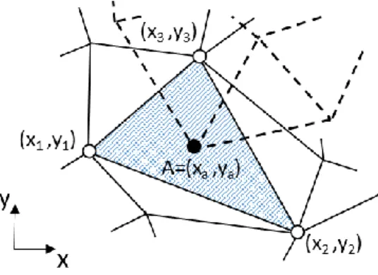
3 DETECTION OF THE FOREGROUND NODES NODE
We consider the conditions under which the nodes of the foreground is present in the ele- ments of the background area. From the definition of the cross product, the node determines whether inside or outside. It is known that determinants D
1, D
2and D
3expressed by Equation (12) must be positive value, if there is node as shown in Figure 2, a = (x
a, y
a), of foreground in an element consists of three nodes, (x
1, y
1), (x
2, y
2), and (x
3, y
3).
a a
a a
a a
a a
a a
a a
y y x x
y y x D x
y y x x
y y x D x
y y x x
y y x D x
1 1
3 3
3
3 3
2 2
2
2 2
1 1
1
(12)
Figure 2: Example of overlapped domain.
4 NUMERICAL EXPERIMENTS
4.1 Comparison of the conventional FEM and the fictitious domain FEM
In the flow field around the cylinder, we compered the analysis using the conventional FEM and the analysis using the fictitious domain FEM. Computational model is shown in Figure 3. In addition, the computational condition for conventional FEM and fictitious do- main FEM is shown in Table 1.
Figure 3: Computational model.
Conventional FEM Fictitious domain FEM
Density 1.00 kg/m
31.00 kg/m
3Kinematic viscosity 0.01 m
2/s 0.01 m
2/s
Time increment Δt 0.001 0.001
Nodes in background domain 1636 1907
Elements in background domain 3116 3716
Nodes in background domain - 331
Elements in foreground domain - 600
Table 1: Computational conditions.
The analysis results are shown in Figures 4-6. Figures 4 and 5 are shown the pressure dis- tribution and the flow velocity vector at T = 10 [s] in the conventional FEM and the fictitious domain FEM. There are no elements inside the moving object in case of the conventional method. On the other hand, in case of the fictitious domain FEM, the physical quantity of the foreground domain is reflected in the background. Therefore, it is seem that the flow velocity vector obtained by the fictitious domain FEM is distributed around the cylinder as same as that obtained by the conventional method. Figure 6 shows the comparison of the time history of the drag force between the conventional FEM and the fictitious domain FEM. From this result, it is found that the result by the fictitious domain FEM is good agreement with that by the conventional FEM.
Figure 4: Pressure and velocity distributions in case of conventional FEM.
Figure 5: Pressure and velocity distributions in case of fictitious domain FEM.
Figure 6: Comparison of time history of drag force between conventional FEM and the fictitious domain FEM.
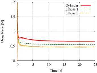
4.2 Comparison of the fluid force for the case of changing the shape of the foreground domain
It is necessary to move the nodes freely in the computational domain, when the appropri- ate shape is obtained such that the drag force minimizes. In this study, the shape expressed by the nodes of the foreground mesh is changed by the solution of the Laplace equation shown in Equation (13) under the boundary condition Equation (14), the comparison of the drag force is carried out in each shape case.
0 0
2 2 2 2
2 2 2 2
y y x
y y
x x
x
(13)
on ˆ
ˆ
i new i
i new i