E End-to-EndSpeechRecognitionSequenceTrainingwithReinforcementLearning

End-to-End Speech Recognition Sequence Training with

Reinforcement Learning

ANDROS TJANDRA

(Nonmember), SAKRIANI SAKTI

(MEMBER, IEEE), AND SATOSHI NAKAMURA

(Fellow, IEEE)

1Nara Institute of Science and Technology (e-mail: [email protected])

2RIKEN, Center for Advanced Intelligence Project AIP, Japan

Corresponding author: Andros Tjandra (e-mail: [email protected]).

ABSTRACT End-to-end sequence modeling has become a popular choice for automatic speech recog- nition (ASR) because of the simpler pipeline compared to the conventional system and its excellent performance. However, there are several drawbacks in the end-to-end ASR model training where the current time-step prediction on the target side are conditioned with the ground truth transcription and speech features. In the inference stage, the condition is different because the model does not have any access to the target sequence ground-truth, thus any mistakes might be accumulated and degrade the decoding result over time. Another issue is raised because of the discrepancy between training and evaluation objective.

In the training stage, maximum likelihood estimation criterion is used as the objective function. However, ASR systems quality is evaluated based on the word error rate via Levenshtein distance. Therefore, we present an alternative for optimizing end-to-end ASR model with one of the reinforcement learning method called policy gradient. The model trained the proposed approach has several advantages: (1) the model simulates the inference stage by free sampling process and uses its own sample as the input, (2) optimize the model with a reward function correlated with the ASR evaluation metric (e.g., negative Levenshtein distance). Based on the result from our experiment, our proposed method significantly improve the model performance compared to a model trained only with teacher forcing and maximum likelihood objective function.

INDEX TERMS End-to-end sequence model, speech recognition, policy gradient optimization, reinforce- ment learning

I. INTRODUCTION

E Nd-to-end sequence modeling has been successfully developed into many different applications, such as:

image captioning [39], [32], machine translation [27], [1], abstractive summarization [17], speech synthesis [33] and speech recognition [2], [3]. Because of their performance and flexibility, sequence-to-sequence models can be applied to many different applications without significant modifica- tion from their original structures. Equipped by recurrent or convolutional neural networks on both the source and target sides, we can encode and conditionally generate a dynamic length sequence directly without extra modules such as fertility [13] for machine translation or duration modeling [40] for speech synthesis. By using sequence-to- sequence architecture, we are able to substitute all the sepa-

rated modules into a single end-to-end system. For example, in the conventional speech recognition system (ASR), there are several modules such as feature extraction, an acoustic model, sub phones and phonemes modeling (GMM-HMM [4], DNN-HMM [7]) and a language model where each of these components is optimized independently. By using end- to-end sequence modeling, we could reduce the effort of constructing sub-modules and making a simpler pipeline.

End-to-end sequence models are typically composed of three different components: encoder, decoder, and attention.

The encoder part extracts features from the source sequence.

The decoder part forms an autoregressive model, which con-

ditionally generates the target sequence step-by-step based on

the previous output, current state, and encoder features. The

attention part is used to calculate the relevance between the

current decoder state and encoder features. For training an autoregressive decoder model, the most popular approach is by using teacher forcing [36]. In teacher forcing, the decoder generates output prediction by using the ground-truth input for current time-step. However, in the inference stage, the decoder has no access to the ground-truth transcription. The decoder needs to rely on its own previous prediction as to the input. As the decoding steps going further, any mistakes from the decoder might be accumulated into the future and the predicted target sequence are diverging from the optimal solution.

Besides the difference between the generation method, the mismatch between the objective in the training and the metric for evaluation could also been problematic [21], [37]. In the training stage, the probability predicted by teacher forc- ing are trained via maximum likelihood estimation (MLE).

Therefore, the loss are usually calculated based on the log- probability for each time-step. However, a models are usu- ally evaluated with different objective or metric such as Levenshtein distance for speech recognition and BLEU [18]

for machine translation. Therefore, optimizing the model parameters with the correct metric is necessary to obtain its best performance in the inference stage.

Here, we introduce an alternative method for optimizing the ASR model by utilizing the concept from reinforcement learning (RL). To be more precise, we apply one of the RL methods called a policy gradient (REINFORCE) [35] to solve the problem arising from teacher forcing and MLE objective.

We assume the ASR autoregressive decoder as an RL agent that produces an action for each time-step, thus we could (1) generate the target sequence transcription with the model’s own prediction instead of teacher forcing, thus simulates the prediction in the inference stage, and (2) construct a reward function that is highly correlated with Levenshtein distance and maximize the expected reward with respect to the agent.

By incorporating the RL method for optimizing our model, the model is still able to be trained end-to-end and also optimized exactly towards ASR evaluation metric.

II. SEQUENCE-TO-SEQUENCE ASR

A sequence-to-sequence (seq2seq) is an end-to-end neural network model that map a dynamic length sequence X = [x

, x

, ..., x

] with length S to another dynamic length sequence Y = [y

, y

, ..., y

] with length T time-step [27].

In the basic form, seq2seq could be formulated as P

(Y |X) parameterized by model parameters θ. In ASR case, we build a seq2seq model that generate a text transcription Y (e.g., character or phoneme) given a speech features X (e.g., MFCC or Mel-spectrogram).

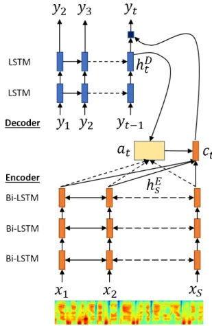
We show our complete structure for seq2seq ASR in Figure 1. There are three main parts in this model: encoder, attention, and decoder modules. Given an input sequence x, the encoder produces a high level representation encoded in the continuous vector H

= [h

, h

, ..., h

]. The attention bridges the information between encoder representation H

and the current decoder’s states h

[1]. Given a pair of

FIGURE 1: Attention-based encoder-decoder architecture.

encoder state h

and decoder state h

, the attention scoring module calculate the relevance score with:

c

=

S

X

s=1

a

(s) h

(1)

a

(s) = Align(h

, h

) (2)

= exp(Score(h

, h

)) P

s=1

exp(Score(h

, h

)) . (3) The alignment between an encoder state and decoder state is calculated with Align(·, ·) function, which is written as a normalized score function Score(·, ·). The scoring function can be written in several different forms:

•

Dot product:

Score(h

, h

) =

M

X

m=1

h

[m] h

[m], (4) where h

, h

∈ R

and without additional free pa- rameter.

•

Bilinear product:

Score(h

, h

) = h

W h

, (5)

where h

∈ R

, h

∈ R

and trainable parameter

W ∈ R

.

•

Multi-layer perceptron (MLP) attention:

Score(h

, h

) = W

tanh(W

h

+ W

h

), (6) where h

∈ R

, h

∈ R

and trainable parameters W

∈ R

, W

∈ R

, W

∈ R

.

We denote M is the hidden unit size from the encoder representation, N is the hidden unit size from the decoder representation and P is the intermediate projection unit size for MLP attention.

The final component for seq2seq is a decoder module. The decoder task is to generate a target discrete sequence Y :

P (Y |X; θ) =

T

Y

t=1

P (y

|c

, h

, y

; θ), (7) where c

is the relevant context generated by the attention module. This equation represent an conditional autoregres- sive model that produces current time-step target probability y

given the previous time-step output y

, a decoder state h

(which consists of a compressed representation for de- coder from time 1 to t − 1) and a context vector c

.

Training seq2seq model mostly done by using maximum likelihood estimation (MLE):

θ

= argmax

θ

P (Y |X ; θ)

= argmax

θ T

Y

t=1

P(y

|c

, h

, y

; θ). (8) Based on the maximum likelihood criterion, we obtained optimal model θ

by minimizing the negative log-likelihood (NLL) calculated by the teacher-forcing generation method:

L

= − log P (y|x; θ),

= − log

T

Y

t=1

P (y

|c

, h

, y

; θ),

= −

T

X

t=1

log P (y

|c

, h

, y

; θ). (9) For each time-step, the teacher-forcing approach generates the label probability based on the ground-truth label at time- t. In Fig. 2, we illustrate the generation process based on the teacher-forcing method. Loss function N LL is described as follows:

N LL(y

, p(y

)) = − X

c

1 {y

= c} log p(y

= c), (10) where p(y

) = P (y

|c

, h

, y

; θ).

However, in the inference stage, since we have no access to the ground-truth transcription, our model must rely on its own previous prediction as input for the current time-step.

We illustrated the decoding process with a greedy approach by taking the label index based on the highest probability mass on p(y

) in Fig. 3.

FIGURE 2: Training stage: generation via teacher-forcing method sets the model input with ground-truth transcrip- tion. For each time-step, decoder generates probability vec- tor p(y

), and we calculate negative log-likelihood between p(y

) and ground-truth y

.

FIGURE 3: Testing/inference stage: decoder doesn’t have access to ground-truth transcription. Therefore, for each time-step t, decoder input depends on model prediction from previous time-step t − 1. For greedy decoding (1- best search), we took the label from highest probability

˜

y

= argmax

yt−1

P (y

|h

) and use selected label y ˜

for current decoder input.

III. REINFORCEMENT LEARNING

In this section, we briefly discuss reinforcement learning, which is an area of machine learning where the agent learns by interacting inside a specific environment. In the learning stage, the agent receives a state and sequentially generates an action through multiple time-steps and eventually the environment returns a reward as a signal feedback for the agent. If agents get a high reward value, it means that they are doing a good job related to their given tasks. Our final goal is to make agents that can choose a series of optimal actions that maximize the reward in that environment.

The RL method can be described formally by the Markov Decision Process (MDP) [28]. Here the agent and environ- ment interact in discrete time-steps t = [1, 2, .., T ]. We formulate a MDP property as a tuple: (S, A, P, R) where

•

S = {S

, S

, .., S

} is a set of the environment’s states

FIGURE 4: Interaction between agent and their environment inside an MDP. Given current state s

, the agent choose an action a

. The environment responds to the selected action and generates a new state s

and a reward r

.

and ∀t ∈ [1..T ], s

∈ S;

•

A = {A

, A

, .., A

} is a set of possible actions for the agent and ∀t ∈ [1..T ], a

∈ A;

•

P : S × S × A → [0, 1] is a state transition probability where P(s

|s, a) is the probability of transitioning to state s

given state s and action a;

•

R : S × A → R is a reward function that returns a value given a state and an action.

In Fig. 4, we illustrated the interaction between an agent and its environment within MDP notation. The MDP process starts from state s

as the initial agent’s state. The initial state s

is defined by the environment (e.g., s

is the location of robot starting point inside certain arena). Based on the initial state s

, the agent chooses actions a

∈ A. Given current state s

∈ S and selected action a

, new state s

is drawn or generated based on state transition probabilities s

∼ P(s

|s

, a

) where s

∈ S. We repeat the process and generate a sequence of states and action from time t ∈ [1..T ]:

s

−→ s

−→ s

−→ ... −−−→

s

−−−→ s

. (11) For each trajectory s

, a

, s

, a

, .., the environment re- turns a series of rewards as a signal feedback:

R(s

, a

) + γR(s

, a

) + γ

R(s

, a

) + .., (12) where γ ∈ [0, 1) is the discount factor for future rewards.

RL’s main target is to optimize an agent that chooses the most optimal actions over time to maximize the expected reward:

E

[R(s

, a

) + γR(s

, a

) + γ

R(s

, a

) + ..]

(13) Policy function π : S → A maps a state to an action.

Given state s

, the policy function returns feasible action a

= π(s

). Value function V

(s) : S → R is defined:

V

(s) = E

[R(s

, a

)+γR(s

, a

)+..|s

= s]. (14)

The value function calculates the expected reward given state s and action a

∼ π taken from policy π. We got the following optimal value function

V

(s) = max

π

V

(s) ∀s ∈ S . (15)

Given optimal value function V

(s), optimal policy π

be- comes

π

= argmax

π

V

(s) ∀s ∈ S . (16)

To extend the value function, a Q-function predicts the ex- pected reward given state-action pair Q : S×A → R defined:

Q

(s, a) = E

[R(s

, a

)+γR(s

, a

)+..|s

= s, a

= a].

(17) The optimal Q-function Q

(s, a) is the maximum action value-function over policies

Q

(s, a) = max

π

Q

(s, a) ∀s ∈ S, ∀a ∈ A. (18) We retrieved best policy π

(s) given state s:

π

(s) = argmax

a

Q

(s, a) ∀s ∈ S. (19) Reinforcement learning can be solved in several ways. First, we can directly optimize policy function π to maximize the expected reward in Eq. 13. Policy gradient [35] is one of the algorithm that optimizes parameterized policy π

with respect to the expected reward. Parameterized policy π

can also be represented with a neural network and optimized di- rectly by first-order optimization such as stochastic gradient descent (SGD). Second, we can find the optimal policy based on Eq. 19 based on the Q-function. Q-learning [34] learns a policy and informs the agent of the expected reward given a certain state and action pair. If we have discrete states and actions, Q-learning can be implemented with a simple table where the state and action pairs are defined by columns and rows and the expected reward value is in the cell. However, when we have high-dimensional states and action spaces, we can replace the table with a function that approximates the Q-function, such as simple linear regression or a deep neural network [22].

IV. POLICY GRADIENT TRAINING FOR SEQUENCE-TO-SEQUENCE ASR

We present our proposed method to incorporate policy opti- mization with seq2seq ASR architecture. First, we present an overview about policy gradient (REINFORCE) optimization strategy. Later, we describe several reward functions that we used to optimize our agent in the reinforcement learning environment.

A. POLICY GRADIENT

Policy gradient is a method based on policy function formu- lation. The policy π

(a|s) optimized directly by adapting the parameters θ to increase the expected reward E[R

|π

] [28].

The parameters θ depends on the function that we use to

approximate the policy. Here, we use deep neural network to parameterized the policy function and θ denotes a collections of neural network weight matrices. To bridge the ASR with reinforcement learning optimization, we need to formulate within an MDP tuple (S, A, P, R), where S is the state space, A is the action space, P is the transition probability between a state to another state, and R is the reward function.

We define our RL agent as a seq2seq ASR model where the agent function is to predict the transcription given a sequence of speech features. We describe the state s

∈ S as a temporary state s

= [c

, h

] from seq2seq decoder at time t ∈ {1..T }. Action state a

∈ A is the discrete output token from the decoder such as character or phoneme symbols. The transition probability P are implied by the operation from RNN cell inside the decoder. Lastly, reward function R are designed to be highly correlated with the quality measure for an ASR system. We provide the detail in Section V.

We assume X

, Y

is a pair between speech features and their groundtruth transcription. The reward R

calcu- lated between the groundtruth Y

and sampled transcrip- tion Y ˜

. We are looking to maximize the expected reward E

[R

|π

] with respect to seq2seq parameters θ where π

(a

|s

) = P(y

|h

, c

; θ) = P (y

|y

, X

; θ).

In order to optimize θ, we calculate the expected reward gradient with respect to the parameters θ:

∇

E

h

R

|π

i

= ∇

Z

P (Y |X

; θ)R

dY

= Z

∇

P(Y |X

; θ)R

dY

= Z

P(Y |X

; θ) ∇

P (Y |X

; θ) P (Y |X

; θ) R

dY

= Z

P(Y |X

; θ)∇

log P(Y |X

; θ)R

dY

= E

h ∇

log P (Y |X

; θ)R

i

≈ 1 M

M

X

m=1

R

∇

log P ( ˜ Y

|X

; θ), (20) where M is the number of samples, Y ˜

∼ P (Y |X

; θ) is the m-th sample from model θ conditioned on input X

, and R

is the calculated reward between ground-truth Y

and sample Y ˜

. From another perspective, Eq. 20 is a bit identical with the gradient from Minimum Risk Training (MRT) [24].

Occasionally using only a single reward signal for a whole sequence of sample Y ˜

m, n) is not sufficient. For example, Eq. 20 can be expanded as:

1 M

M

X

m=1 M

X

m=1

R

∇

X

t=1

log P (˜ y

|X

; θ)

(21) which is we distribute the sequence reward R

to all time-step equally. There might be a sub-optimal case where

the reward is negative caused by several time-step action, but we penalize all time-step with negative reward instead.

Therefore, we could substitute the reward R

with time- distributed reward R

∈ R , ∀t ∈ {1..T }. The reward R

might have different value between different time-step, thus it could provide more informative feedback for each time-step.

Mathematically, we substitute Eq. 20 t = [1, .., T ] with:

∇

E

"

X

t=1

R

|π

#

= ∇

Z

P (Y |X

; θ)

T

X

t=1

R

! dY

= Z

P(Y |X

; θ) ∇

P (Y |X

; θ) P(Y |X

; θ)

T

X

t=1

R

! dY

= Z

P(Y |X

; θ)∇

log P(Y |X

; θ)

T

X

t=1

R

! dY

= E

"

X

t=1

R

!

∇

log P (Y |X

; θ)

#

= E

"

X

t=1

R

!

X

t=1

∇

log P(y

|y

, X

; θ)

#

≈ E

"

X

t=1

R

∇

log P (y

|y

, X

; θ)

#

(22)

≈ 1 M

M

X

m=1 T(m)

X

t=1

R

∇

log P (˜ y

| y ˜

, X

; θ),

(23) where T is the length of transcription Y , R

is the gener- alized reward based on the current state and action at time- t. In Eq. 23, R

is the reward from m-th sample, time- step t-th and compared with n-th utterance groundtruth, and T (m) denotes the sample Y ˜

length. To calculate the expected reward from Eq. 20 and Eq. 23, we need to integrate all possible transcription across random variable Y . It is unrealistic because the search space are growing exponential for each time-step. Therefore, we do Monte-carlo sampling M times per sequence Y ˜

∼ P (Y |X

; θ) for each utterance X

to get an approximated expected reward.

To summarize our explanation, we compared the differ-

ences between teacher-forcing and policy gradient loss cal-

culation from Figs. 2 and 5. In the teacher-forcing method,

the model predictions are generated based on the ground-

truth transcription. However, in the policy gradient method,

first we sample M sequences by Monte Carlo sampling and

stop after getting an </s> symbol. Then we calculate dis-

counted reward R

for each time-step based on the future

rewards. We provide pseudocode to complete our explanation

in Alg. 1.

FIGURE 5: Policy gradient set decoder input to be condi- tioned on its own prediction sampled from previous time- step to predict current time-step output probability. There- fore, decoder doesn’t rely on a ground-truth transcription like teacher-forcing method. Expected rewards for model transcription are approximated by the average from multiple sample trajectories.

V. REWARD CONSTRUCTION FOR ASR TASKS

One important component for optimizing an agent using an reinforcement learning approach is to design a good reward function that closely corresponds to the metric that we used to evaluate our agent performance. In our case, our agent is ASR systems that were evaluated based on the edit-distance or the Levenshtein distance algorithm. Therefore, we composed our reward function with a modified edit-distance algorithm and divided the reward into two different types:

A. SENTENCE-LEVEL REWARD

Based on Eq. 20, we need to calculate the reward by com- paring ground-truth transcription Y

and sampled tran- scription Y ˜

. In this case, we designed reward function R( ˜ Y

, Y

) to calculate R

:

R

= R( ˜ Y

, Y

) = − ED( ˜ Y

, Y

)

|Y

| , (24) where ED(·, ·) is an edit-distance function. In practice, we would like to minimize the edit-distance between the sample and the ground-truth transcription. However, for the reinforcement learning environment, we design a reward function with the opposite output. For example, if our model produces two samples, Y ˜

and Y ˜

, the first Y ˜

is “closer" to Y

than the second Y ˜

, then the reward function must fulfill: R( ˜ Y

, Y

) > R( ˜ Y

, Y

).

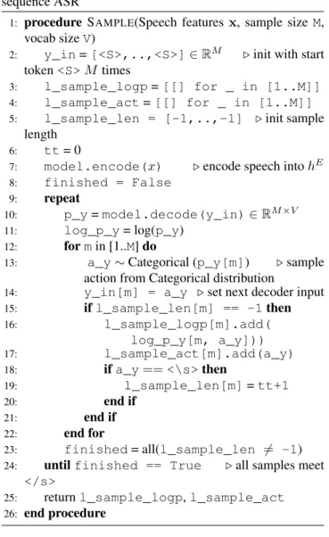
Algorithm 1 Pseudocode for sampling text on sequence-to- sequence ASR

1:

procedure S

(Speech features x, sample size M, vocab size V)

2:

y_in = [<S>,..,<S>] ∈ R

. init with start token <S> M times

3:

l_sample_logp = [[] for _ in [1..M]]

4:

l_sample_act = [[] for _ in [1..M]]

5:

l_sample_len = [-1,..,-1] . init sample length

6:

tt = 0

7:

model.encode(x) . encode speech into h

8:

finished = False

9:

repeat

10:

p_y = model.decode(y_in) ∈ R

11:

log_p_y = log(p_y)

12:

for m in [1..M] do

13:

a_y ∼ Categorical (p_y[m]) . sample action from Categorical distribution

14:

y_in[m] = a_y . set next decoder input

15:

if l_sample_len[m] == -1 then

16:

l_sample_logp[m].add(

log_p_y[m, a_y]))

17:

l_sample_act[m].add(a_y)

18:

if a_y == <\s> then

19:

l_sample_len[m] = tt+1

20:

end if

21:

end if

22:

end for

23:

finished = all(l_sample_len 6= -1)

24:

until finished == True . all samples meet

</s>

25:

return l_sample_logp, l_sample_act

26:

end procedure

Therefore, we multiply the edit-distance result by -1 to fulfill the requirement of the reward function.

Since the REINFORCE gradient estimator is usually too noisy and might hinder our learning process, there are several tricks to reduce the variance [6], [15]. Here we normalize reward R

:

µ

= 1 M

M

X

m=1

R( ˜ Y

, Y

)

σ

= 1 M

M

X

m=1

R( ˜ Y

, Y

) − µ

R

= R( ˜ Y

, Y

) − µ

σ

. (25)

We normalize our reward across M samples into zero mean

and unit variance. We provide the pseudocode for calculating

sentence-level reward in Algorithm 2.

B. TOKEN-LEVEL REWARD

Rather than having only a single reward attributed to the whole sequence, we could also construct a better reward function which give a feedback for every time-step. Here we design a reward function that could provide an intermediate reward before the sample transcription finished. This reward function R( ˜ Y , Y

, t) calculate R

by utilizing the edit- distance algorithm. We define reward R( ˜ Y , Y

, t):

R( ˜ Y

, Y

, t) =



 

 



 

 



|Y

| − ED( ˜ Y

, Y

) if t = 1 ED( ˜ Y

, Y

) − ED( ˜ Y

, Y

) if 1 < t < T

−ED( ˜ Y

, Y

) if t = T (26) where ED(·, ·) is the edit-distance function between two transcriptions, Y ˜

is a substring of Y ˜

from index 1 to t, |Y

| is the ground-truth length, and T is the sample transcription Y ˜

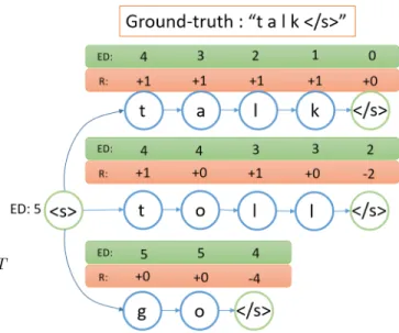
length. Intuitively, we calculate whether the current new transcription at time-t decreases the edit- distance compared to previous transcriptions and multiply it by -1 for a positive reward if our new edit-distance at time t is smaller than the previous t − 1 edit-distance. Also, at the end-of-sentence at time-T , we give a penalty based on the final edit-distance between the sample and the ground-truth transcription. In Fig. 6, we illustrate our reward scoring at each time-step from different trajectory samples.

In most cases, the current selected action affects future states and actions as well. Therefore, we should also account for some of the future rewards in the current time-step.

Reward R

can be written:

R

=R( ˜ Y

, Y

, t)

+ γR( ˜ Y

, Y

, t + 1) + γ

R( ˜ Y

, Y

, t + 2) + ...

+ γ

R( ˜ Y

, Y

, T ), (27) where γ is the discount factor.

Additionally, since the REINFORCE estimator has high variance and could cause instability in the training stage, we apply the following normalization for reward R

:

R

=



 

 

 

 

 

 

R( ˜ Y

, Y

, t) − µ

σ

if 1 ≤ t < T

R( ˜ Y

, Y

, t) − µ

σ

if t = T , (28) where µ

, σ

is the reward mean and standard devia- tion for all samples at the t-th timestep, µ

, σ

is the reward mean and standard deviation for all the samples

FIGURE 6: Based on Eq. 26, we provide an example for how to calculate the reward for each sample trajectory.

at the end of the transcription (denoted with <\s>), and T is the sample transcription Y ˜

length. We separate the mean and the standard deviations between <\s> and non-

<\s> labels because the reward function (Eq. 26) has differ- ent ways to calculate the reward. We provide the pseudocode for calculating token-level reward in Algorithm 3.

Algorithm 2 Pseudo-code for policy gradient with sentence- level reward R

1:

procedure L

PGS

(Speech features x, ground-truth text y_gold, sample size M, vocab size V)

2:

l_s_logp, l_s_act = Sample(x, M, V) . Algorithm 1

3:

l_r = []

4:

for m in [1..M] do

5:

# Calculate reward between ground-truth and each sample

6:

l_r.add(R(y_gold, l_s_act[m])) . Eq. 24

7:

end for

8:

# Reward normalization

9:

l_r = (l_r - mean(l_r)) / std(l_r) . Eq. 25

10:

# Calculate loss and update θ

model

11:

L = 0

12:

for m in [1..M] do

13:

for t in [1..len(l_s_act[m])] do

14:

L += -l_s_logp[m, t] * l_r[m]

15:

end for

16:

end for

17:

θ

= Optim(θ

, ∇

L) . update ASR parameters

18:

end procedure

VI. EXPERIMENT

Algorithm 3 Pseudocode for policy gradient with token-level reward R

1:

procedure L

PGT

(Speech features x, ground- truth text y_gold, sample size M, discount factor γ, vocab size V)

2:

l_s_logp, l_s_act = Sample(x, M, V) . Algorithm 1

3:

l_r = [[] for _ in [0..M]]

4:

for m in [1..M] do

5:

for t in [1..len(l_s_act[m])] do

6:

# Calculate reward between ground-truth and each sample at time-t

7:

l_r[m].add(R(l_s_act[m],

y_gold, t)) . Eq. 26

8:

end for

9:

end for

10:

# Calculate discounted reward

11:

for m in [1..M] do

12:

R = 0

13:

for t in [len(l_s_act[m]) .. 1] do

14:

R = l_r[m, t] + γ * R

15:

l_r[m, t] = R

16:

end for

17:

end for

18:

# Reward normalization

19:

l_r = normalization(l_r) . Eq. 28

20:

# Calculate loss and update θ

model

21:

for m in [1..M] do

22:

for t in [1..len(l_s_act[m])] do

23:

L += -l_s_logp[m, t] * l_r[m, t]

24:

end for

25:

end for

26:

θ

= Optim(θ

, ∇

L) . update ASR parameters

27:

end procedure

A. SPEECH DATASET AND FEATURE EXTRACTION

We evaluate our proposed method using Wall Street Journal dataset (WSJ) [19]. Following Kaldi s5 recipe [20], we use same training, validation and test sets partition. For the training, we a smaller set (train_si84) for preliminary and faster experiment, then later we use full set (train_si284). The speech features are computed with 80-dimension log Mel- filterbank with 25 ms window width and 10 ms window step.

The text transcription are tokenized into characters, which contains alphabet, space, dashes, periods, apostrophes, noise and end-of-sentence (</s>). We describe the details for such as number of utterances, duration and unique speakers for each set on WSJ in Table 1.

B. MODEL ARCHITECTURE

Our encoder input is a sequence of Mel-frequency spec- trogram with 80 dimensions. For each frame, the input is projected by a dense linear layer with 512 output units and transformed by leaky rectifier unit (LeakyReLU) [38] as the

TABLE 1: WSJ subset information

Subset Utterances Duration Speakers

train_si84 7138 16 h 83

train_s284 38154 80 h 282

eval_dev93 503 65 m 10

eval_test92 333 42 m 8

non-linear activation function. Later, the output from dense linear layer was processed by three bi-directional LSTMs [8]

(bi-LSTM) with 512 hidden units (256 hidden units for each direction). We apply hierarchical sub-sampling [5], [2] by a factor of 2 for all bi-LSTM output and the final encoder states has T /8 length compared to the original speech features. This trick is useful to reduce the computation time and memory usage for seq2seq model.

Our decoder has an autoregressive form which takes the character output from the previous time-step as the current time-step input. Every character is projected by a continu- ous vector via character embedding with 128 dimensions.

Later, one uni-directional LSTM with 512 units project the character vector. The attention module with MLP scorer (256 units projection layer) calculates the context vector c

, concatenated with the LSTM output and finally projected into a categorical probability distribution with a softmax layer. To optimize our seq2seq ASR model, we use Adam [11] with learning rate lr = 0.0005.

We have two steps of training seq2seq ASR. First, we pre- train seq2seq ASR by minimizing NLL criterion (Eq. 10) via teacher forcing generation until the loss is stable and converged. Later, we continue the training by summing the RL objective with the NLL criterion at the same time until the character error rate (CER) in the dev set stops decreasing.

We use beam-search (beam-size = 5) decoding to transcript the speech utterance in the testing step. Each beam score is calculated by their log probability log P(Y |X ; θ) and divided by the hypothesis length to prevent the top-K beams promoting shorter hypothesis. In this work, we did not utilize any lexicon dictionary or language model. We use Pytorch

library to implement our model and loss function.

1PyTorch https://github.com/pytorch/pytorch/

VII. RESULTS AND DISCUSSION

TABLE 2: Character error rate (CER) report from WSJ train_si84 set (small set), comparing the result between base- line (without RL) and proposed method (NLL + RL). All decoding results were produced without additional language model or lexicon dictionary.

Models Results

WSJ-SI84 CER (%)

NLL

CTC [10] 20.34 %

Seq2Seq Content [10] 20.06 % Seq2Seq Location [10] 17.01 % Joint CTC+Att (MTL) [10] 14.53 %

Seq2Seq (ours) 17.68 %

NLL + RL

Seq2Seq + RL

(sentence-level

16.88 % Seq2Seq + RL

(sentence-level

15.38 % Seq2Seq + RL

(sentence-level

15.21 % Seq2Seq + RL

(token-level

,

15.17 % Seq2Seq + RL

(token-level

,

15.34 % Seq2Seq + RL

(token-level

,

14.75 % Seq2Seq + RL

(token-level

,

15.08 % Seq2Seq + RL

(token-level

,

14.45 % Seq2Seq + RL

(token-level

,

14.29 % Seq2Seq + RL

(token-level

,

14.99 % Seq2Seq + RL

(token-level

,

14.25 % Seq2Seq + RL

(token-level

,

13.92 %

Table 2 shows the ASR performance on the WSJ-SI84. Here, we compare our proposed model (NLL + RL) with the baseline (without RL). Our baseline model is an attention encoder-decoder that was only trained with the NLL objec- tive. In addition, we also compared our results with several published models, including CTC, standard seq2seq, and the Joint CTC-Attention model trained with the NLL objective.

The main difference between our seq2seq model with others is that our decoder calculates the attention probability and context vector based on the current hidden state instead of the previous hidden state. Furthermore, we also reused the previous context vector by concatenating it with the input embedding vector.

We ran various experiments with different scenarios:

•

Reward types:

1) sentence-level reward (Sec. V-A) 2) token-level reward (Sec. V-B)

•

Sample sizes:

FIGURE 7: CER (%) comparisons between different sample sizes M

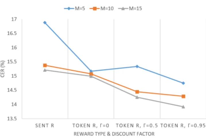
FIGURE 8: CER (%) comparison between different reward types and discount factors γ.

1) M = 5 2) M = 10 3) M = 15

•

Discount factors (for token-level reward):

1) γ = 0 2) γ = 0.5 3) γ = 0.95

To show the effect of different sample sizes, we plotted the performances into different lines with respect to the CER in Fig. 7. From another perspective, we also provided Fig. 8 to compare the performances within different reward formulations and discount factors.

Based on the result in Table 2, we observed the following:

1) Increasing sample size M from 5 to 10 and 10 to

15 generally improved the performance. Unfortunately,

the training time also increased linearly with sample

size M .

2) Token-level reward improved the performance more than the model trained with the sentence-level reward.

3) Discount factor γ = 0.95 provided a better result than γ = 0.5 and γ = 0.0 in most cases.

Next we extended our experiment on WSJ train_si284, which is much larger than train_si84. Since our previous ob- servation about the train_si84 dataset concluded that sample M = 15 gave a better result than any smaller sample size, we fixed our sample size to M = 15.

TABLE 3: Character error rate (CER) report from WSJ train_si284 set (large set), comparing the result between baseline (without RL) and proposed method (NLL + RL). All decoding results were produced without additional language model or lexicon dictionary.

Models Results

WSJ-SI284 CER (%)

MLE

CTC [10] 8.97 %

Seq2Seq Content [10] 11.08 % Seq2Seq Location [10] 8.17 % Joint CTC+Att (MTL) [10] 7.36 %

Seq2Seq (ours) 7.69%

MLE+RL

Seq2Seq + RL

(sentence-level

7.26%

Seq2Seq + RL

(token-level

,

6.64 % Seq2Seq + RL

(token-level

,

6.37 % Seq2Seq + RL

(token-level

,

6.10 %

We provide the result from WSJ train_si284 in Table 3.

From the table, we could observe that the combination be- tween NLL teacher forcing and RL objective significantly improve the seq2seq ASR performance compared to a model trained by NLL teacher forcing only. For both train_si84 and train_si284 dataset, the best discount factor for token-level reward is γ = 0.95.

VIII. RELATED WORK

Reinforcement learning is one of important types of machine learning where an agent that interacts with its environment learns how to maximize the rewards using feedback signals.

Reinforcement learning have been successfully applied in many applications, including building an agent that can learn how to behave in environment and play a game without having any explicit knowledge [16], [25], control tasks in robotics [12], and dialogue system agents [26], [14].

Not limited to those areas, reinforcement learning has also been adopted for improving end-to-end deep learning architecture. To date, Ranzato et al. [21] proposed to com- bine REINFORCE with an MLE training objective called MIXER. In the early stage of training, the first s steps were trained with MLE and the remaining T-s steps with REINFORCE. They decreased s as the training progress

over time. By using REINFORCE, they trained the model using non-differentiable task-related rewards (e.g., BLEU for machine translation). In this paper, we did not need to deal with any scheduling or mix any sampling with the teacher- forcing ground-truth. Furthermore, MIXER did not sample multiple sequences based on the REINFORCE Monte Carlo approximation.

In machine translation tasks, Shen et al. [24] could im- prove the neural machine translation (NMT) model using Minimum Risk Training (MRT). A Google NMT [37] sys- tem combined MLE and MRT objectives to achieve better results. In ASR tasks, Shanon et al. [23] performed WER optimization by sampling paths from the lattices that were used during sMBR training, which seemingly resembles the REINFORCE algorithm. But the work was only applied to a CTC-based model. From a probabilistic perspective, MRT formulation resembles the expected reward formulation used in reinforcement learning. Here, MRT formulation equally distributed the sentence-level loss into all of the time-steps in the sample. To the best of our knowledge, we are the first to publish the work on optimizing attention-based encoder- decoder ASR with reinforcement learning approach [31].

Later on, similar work is also published by Karita et al. [9].

The main difference between our work and their work is the design of the reward function and the sampling process.

This paper is the extension from our previous work [30], [29]. On this paper, we provide a more detailed description of our proposed method and more comparison to observe the correlation between RL hyperparameters and the perfor- mance improvement. Finally, we found that using token-level reward is more effective for training our system compared to sentence-level reward or loss. Therefore, we proposed a tem- poral structure and applied token-level reward R

. Our results demonstrate that we improved our performance significantly compared to the baseline system.

IX. CONCLUSION

This paper introduced an alternative strategy for training end-to-end ASR models by integrating an idea from rein- forcement learning. Our proposed method integrates: (1) the power of sequence-to-sequence approaches to learn mapping between speech signals and text transcription; and (2) the strength of reinforcement learning to directly optimize the model with ASR performance metrics. Here, several different scenarios for training with RL-based objectives are explored with various reward functions, sample sizes, and discount factors. Experimental results reveal that by combining RL- based objectives with MLE objectives, our model perfor- mance could significantly improve in comparison to the model that just trained with MLE objectives. The best system achieved up to 6.10% CER in WSJ-SI284 using token-level rewards, sample size M = 15, and discount factor γ = 0.95.

X. ACKNOWLEDGEMENT

Part of this work was supported by JSPS KAKENHI Grant

Numbers JP17H06101 and JP17K00237.

REFERENCES

[1] D. Bahdanau, K. Cho, and Y. Bengio, “Neural machine translation by jointly learning to align and translate,” arXiv preprint arXiv:1409.0473, 2014.

[2] D. Bahdanau, J. Chorowski, D. Serdyuk, P. Brakel, and Y. Bengio, “End- to-end attention-based large vocabulary speech recognition,” in Proc.

ICASSP, 2016. IEEE, 2016, pp. 4945–4949.

[3] W. Chan, N. Jaitly, Q. Le, and O. Vinyals, “Listen, attend and spell: A neural network for large vocabulary conversational speech recognition,” in Acoustics, Speech and Signal Processing (ICASSP), 2016 IEEE Interna- tional Conference on. IEEE, 2016, pp. 4960–4964.

[4] M. Gales, S. Young et al., “The application of hidden markov models in speech recognition,” Foundations and TrendsR in Signal Processing, vol. 1, no. 3, pp. 195–304, 2008.

[5] A. Graves et al., Supervised sequence labelling with recurrent neural networks. Springer, 2012, vol. 385.

[6] E. Greensmith, P. L. Bartlett, and J. Baxter, “Variance reduction techniques for gradient estimates in reinforcement learning,” Journal of Machine Learning Research, vol. 5, no. Nov, pp. 1471–1530, 2004.

[7] G. Hinton, L. Deng, D. Yu, G. Dahl, A.-r. Mohamed, N. Jaitly, A. Senior, V. Vanhoucke, P. Nguyen, B. Kingsbury et al., “Deep neural networks for acoustic modeling in speech recognition,” IEEE Signal processing magazine, vol. 29, 2012.

[8] S. Hochreiter and J. Schmidhuber, “Long short-term memory,” Neural computation, vol. 9, no. 8, pp. 1735–1780, 1997.

[9] S. Karita, A. Ogawa, M. Delcroix, and T. Nakatani, “Sequence training of encoder-decoder model using policy gradient for end- to-end speech recognition,” in 2018 IEEE International Conference on Acoustics, Speech and Signal Processing (ICASSP), April 2018, pp. 5839–5843.

[10] S. Kim, T. Hori, and S. Watanabe, “Joint CTC-attention based end-to- end speech recognition using multi-task learning,” in Acoustics, Speech and Signal processing (ICASSP), 2017 IEEE International Conference on.

IEEE, 2017.

[11] D. Kingma and J. Ba, “Adam: A method for stochastic optimization,”

arXiv preprint arXiv:1412.6980, 2014.

[12] J. Kober and J. Peters, “Reinforcement learning in robotics: A survey,” in Reinforcement Learning. Springer, 2012, pp. 579–610.

[13] P. Koehn, Statistical machine translation. Cambridge University Press, 2009.

[14] J. Li, W. Monroe, A. Ritter, M. Galley, J. Gao, and D. Jurafsky,

“Deep reinforcement learning for dialogue generation,” arXiv preprint arXiv:1606.01541, 2016.

[15] A. Mnih and K. Gregor, “Neural variational inference and learning in belief networks,” in Proceedings of the 31st International Conference on International Conference on Machine Learning-Volume 32. JMLR. org, 2014, pp. II–1791.

[16] V. Mnih, K. Kavukcuoglu, D. Silver, A. A. Rusu, J. Veness, M. G.

Bellemare, A. Graves, M. Riedmiller, A. K. Fidjeland, G. Ostrovski, S. Petersen, C. Beattie, A. Sadik, I. Antonoglou, H. King, D. Kumaran, D. Wierstra, S. Legg, and D. Hassabis, “Human-level control through deep reinforcement learning,” Nature, vol. 518, no. 7540, pp. 529–533, 02 2015. [Online]. Available: http://dx.doi.org/10.1038/nature14236 [17] R. Nallapati, B. Zhou, C. dos Santos, C. Gulcehre, and B. Xiang, “Abstrac-

tive text summarization using sequence-to-sequence rnns and beyond,” in Proceedings of The 20th SIGNLL Conference on Computational Natural Language Learning, 2016, pp. 280–290.

[18] K. Papineni, S. Roukos, T. Ward, and W.-J. Zhu, “Bleu: a method for automatic evaluation of machine translation,” in Proceedings of the 40th annual meeting on association for computational linguistics. Association for Computational Linguistics, 2002, pp. 311–318.

[19] D. B. Paul and J. M. Baker, “The design for the Wall Street Journal- based CSR corpus,” in Proceedings of the Workshop on Speech and Natural Language, ser. HLT ’91. Stroudsburg, PA, USA: Association for Computational Linguistics, 1992, pp. 357–362. [Online]. Available:

http://dx.doi.org/10.3115/1075527.1075614

[20] D. Povey, A. Ghoshal, G. Boulianne, L. Burget, O. Glembek, N. Goel, M. Hannemann, P. Motlicek, Y. Qian, P. Schwarz, J. Silovsky, G. Stemmer, and K. Vesely, “The Kaldi speech recognition toolkit,” in IEEE 2011 Workshop on Automatic Speech Recognition and Understanding. IEEE Signal Processing Society, Dec. 2011, iEEE Catalog No.: CFP11SRW- USB.

[21] M. A. Ranzato, S. Chopra, M. Auli, and W. Zaremba, “Sequence level training with recurrent neural networks,” arXiv preprint arXiv:1511.06732, 2015.

[22] J. Schmidhuber, “Deep learning in neural networks: An overview,” Neural networks, vol. 61, pp. 85–117, 2015.

[23] M. Shannon, “Optimizing expected word error rate via sampling for speech recognition,” arXiv preprint arXiv:1706.02776, 2017.

[24] S. Shen, Y. Cheng, Z. He, W. He, H. Wu, M. Sun, and Y. Liu, “Minimum risk training for neural machine translation,” in Proceedings of the 54th Annual Meeting of the Association for Computational Linguistics, ACL 2016, August 7-12, 2016, Berlin, Germany, Volume 1: Long Papers, 2016.

[Online]. Available: http://aclweb.org/anthology/P/P16/P16-1159.pdf [25] D. Silver, A. Huang, C. J. Maddison, A. Guez, L. Sifre, G. Van Den Driess-

che, J. Schrittwieser, I. Antonoglou, V. Panneershelvam, M. Lanctot et al.,

“Mastering the game of go with deep neural networks and tree search,”

Nature, vol. 529, no. 7587, pp. 484–489, 2016.

[26] S. P. Singh, M. J. Kearns, D. J. Litman, and M. A. Walker, “Reinforcement learning for spoken dialogue systems,” in Advances in Neural Information Processing Systems, 2000, pp. 956–962.

[27] I. Sutskever, O. Vinyals, and Q. V. Le, “Sequence to sequence learning with neural networks,” in Advances in neural information processing systems, 2014, pp. 3104–3112.

[28] R. S. Sutton and A. G. Barto, Introduction to Reinforcement Learning, 1st ed. Cambridge, MA, USA: MIT Press, 1998.

[29] A. Tjandra, S. Sakti, and S. Nakamura, “Sequence-to-sequence asr opti- mization via reinforcement learning,” in 2018 IEEE International Confer- ence on Acoustics, Speech and Signal Processing (ICASSP), April 2018, pp. 5829–5833.

[30] ——, “Attention-based wav2text with feature transfer learning,” in 2017 IEEE Automatic Speech Recognition and Understanding Workshop, ASRU 2017, Okinawa, Japan, December 16-20, 2017, 2017, pp. 309–315.

[Online]. Available: https://doi.org/10.1109/ASRU.2017.8268951 [31] ——, “Sequence-to-sequence asr optimization via reinforcement learn-

ing,” arXiv preprint arXiv:1710.10774, 2017.

[32] O. Vinyals, A. Toshev, S. Bengio, and D. Erhan, “Show and tell: A neural image caption generator,” in Proceedings of the IEEE conference on computer vision and pattern recognition, 2015, pp. 3156–3164.

[33] Y. Wang, R. Skerry-Ryan, D. Stanton, Y. Wu, R. J. Weiss, N. Jaitly, Z. Yang, Y. Xiao, Z. Chen, S. Bengio et al., “Tacotron: Towards end-to- end speech synthesis,” arXiv preprint arXiv:1703.10135, 2017.

[34] C. J. Watkins and P. Dayan, “Q-learning,” Machine learning, vol. 8, no.

3-4, pp. 279–292, 1992.

[35] R. J. Williams, “Simple statistical gradient-following algorithms for con- nectionist reinforcement learning,” Machine learning, vol. 8, no. 3-4, pp.

229–256, 1992.

[36] R. J. Williams and D. Zipser, “A learning algorithm for continually running fully recurrent neural networks,” Neural computation, vol. 1, no. 2, pp.

270–280, 1989.

[37] Y. Wu, M. Schuster, Z. Chen, Q. V. Le, M. Norouzi, W. Macherey, M. Krikun, Y. Cao, Q. Gao, K. Macherey et al., “Google’s neural ma- chine translation system: Bridging the gap between human and machine translation,” arXiv preprint arXiv:1609.08144, 2016.

[38] B. Xu, N. Wang, T. Chen, and M. Li, “Empirical evaluation of rectified activations in convolutional network,” arXiv preprint arXiv:1505.00853, 2015.

[39] K. Xu, J. Ba, R. Kiros, K. Cho, A. Courville, R. Salakhudinov, R. Zemel, and Y. Bengio, “Show, attend and tell: Neural image caption generation with visual attention,” in International Conference on Machine Learning, 2015, pp. 2048–2057.

[40] H. Zen, K. Tokuda, and A. W. Black, “Statistical parametric speech synthesis,” Speech Communication, vol. 51, no. 11, pp. 1039–1064, 2009.

ANDROS TJANDRAreceived a B.E. degree in Computer Science (cum laude) from the Faculty of Computer Science, Universitas Indonesia, In- donesia in 2014 and a M.S. (cum laude) in 2015 from the same faculty and university. He is cur- rently a doctoral student at the Graduate School of Information Science, Nara Institute of Technol- ogy, Japan. He is a student member of ASJ. His research interests include machine learning (deep learning), speech recognition, speech synthesis, and natural language processing.

SAKRIANI SAKTI is a research associate pro- fessor at the Augmented Human Communication Laboratory, NAIST, Japan, as well as a research scientist at RIKEN, Center for Advanced Intel- ligent Project AIP, Japan. She received her B.E.

degree in Informatics (cum laude) from Bandung Institute of Technology, Indonesia, in 1999. In 2000, she received DAAD-Siemens Program Asia 21st Century Award to study in Communication Technology, University of Ulm, Germany, and re- ceived her MSc degree in 2002. During her thesis work, she also worked with Speech Understanding Department, aimlerChrysler Research Center, Ulm, Germany. Between 2003-2009, she worked as a researcher at ATR SLC Labs, Japan, and during 2006-2011, she worked as an expert researcher at NICT SLC Groups, Japan. While working with ATR-NICT, Japan, she continued her study (2005-2008) at University of Ulm, Germany, and received her PhD degree in 2008. She was actively involved in collaboration activities such as Asian Pacific Telecommunity Project (2003-2007), A- STAR and U-STAR (2006-2011). In 2009-2011, she served as a visiting professor of Computer Science Department, University of Indonesia (UI), Indonesia. From 2011, she has been an assistant professor at the Augmented Human Communication Laboratory, NAIST, Japan. She served also as a visiting scientific researcher of INRIA Paris-Rocquencourt, France, in 2015- 2016, under “JSPS Strategic Young Researcher Overseas Visits Program for Accelerating Brain Circulation”. In 2011-2017, she served as an assistant professor at the Augmented Human Communication Laboratory, NAIST, Japan. Now she is a research associate professor at the Augmented Human Communication Laboratory, NAIST, Japan, as well as a research scientist at RIKEN, Center for Advanced Intelligent Project AIP, Japan. She is a member of JNS, SFN, ASJ, ISCA, IEICE and IEEE.

SATOSHI NAKAMURAis Professor at the Grad- uate School of Information Science, Nara Institute of Science and Technology, Japan, Honorarpro- fessor of Karlsruhe Institute of Technology, Ger- many, and ATR Fellow. He received his B.S. from Kyoto Institute of Technology in 1981 and Ph.D.

from Kyoto University in 1992. He was Associate Professor of Graduate School of Information Sci- ence at Nara Institute of Science and Technology in 1994-2000. He was Director of ATR Spoken Language Communication Research Laboratories in 2000-2008 and Vice president of ATR in 2007-2008. He was Director General of Keihanna Research Laboratories and the Executive Director of Knowledge Creating Communication Research Center, National Institute of Information and Communications Technology, Japan in 2009-2010. He is currently Director of Augmented Human Communication laboratory and a full professor of Graduate School of Information Science at Nara Institute of Science and Technology. He is interested in modeling and systems of speech-to-speech translation and speech recognition. He is one of the leaders of speech- to-speech translation research and has been serving for various speech- to-speech translation research projects in the world including C-STAR, IWSLT and A-STAR. He received Yamashita Research Award, Kiyasu Award from the Information Processing Society of Japan, Telecom System Award, AAMT Nagao Award, Docomo Mobile Science Award in 2007, ASJ Award for Distinguished Achievements in Acoustics. He received the Commendation for Science and Technology by the Minister of Education, Science and Technology, and the Commendation for Science and Tech- nology by the Minister of Internal Affairs and Communications. He also received LREC Antonio Zampoli Award 2012. He has been Elected Board Member of International Speech Communication Association, ISCA, since June 2011, IEEE Signal Processing Magazine Editorial Board Member since April 2012, IEEE SPS Speech and Language Technical Committee Member since 2013, and IEEE Fellow since 2016.