175978-1-4799-7291-3/15/$31.00 ©2015 IEEEASRU 2015

STOCHASTIC GRADIENT VARIATIONAL BAYES FOR DEEP LEARNING-BASED ASR Andros Tjandra ¹ , Sakriani Sakti ² , Satoshi Nakamura ² , Mirna Adriani ¹

1 Faculty of Computer Science, Universitas Indonesia, Indonesia

2 Graduate School of Information Science, Nara Institute of Science and Technology, Japan

[email protected], [email protected], {ssakti,s-nakamura}@is.naist.jp

ABSTRACT

Many successful methods for training deep neural networks (DNN) rely on an unsupervised pretraining algorithm. It is particularly effective when the number of labeled training samples is not large enough, because pretraining method helps to initialize the parameter values in the appropriate range near a local good minimum, for further discriminative finetuning. However, while the improvement is impressive, training DNN is difficult because the objective function of DNN is highly non-convex function of the parameters. To avoid placing the parameter that generalizes poorly, a robust generative modelling is necessary. This paper explore an al- ternative of generative modelling for pretraining DNN-based acoustic modelling using Stochastic Gradient Variational Bayes (SGVB) within autoencoder framework called Varia- tional Bayes Autoencoder (VBAE). It performs an efficient approximate inference and learning with directed proba- bilistic graphical models. During fine-tuning, probabilistic encoder parameters with latent variable components are then used in discriminative training for acoustic model. Here, we investigate the performances of DNN-based acoustic model using the proposed pretrained VBAE in comparison with widely used pretraining algorithms like Restricted Boltz- mann Machine (RBM) and Stacked Denoising Autoencoder (SDAE). The results reveal that VBAE pretraining with Gaus- sian latent variables gave the best performance.

Index Terms— acoustic model, deep neural network, variational bayes, autoencoder

1. INTRODUCTION

Automatic Speech Recognition (ASR) has changed dramat- ically in recent years. Previously, the standard ASR frame- work used Hidden Markov Model (HMM) to model the speech state transition/sequence [1] and Gaussian Mixture Model (GMM) to model each acoustic state on HMM from speech features [2]. GMMs hold such advantages as being easily fit into data using EM algorithms (especially with diag- onal covariance matrix) and if they have enough parameters, they can approximate any distribution very well. However, GMMs also have disadvantages which is statistically ineffi-

cient for modelling highly correlated data due to the indepen- dent assumption of diagonal covariance. Furthermore, EM algorithms for GMM often suffer from overfitting when the component number is not adequate with the data amount.

Various state-of-the-art performances produced by deep learning have revitalized the use of various kinds of neural network architecture in ASR. A Deep Neural Network (DNN) based ASR has gained popularity in recent years, driven by bigger performance improvements than such to the previous common methods like GMM/HMM [3]. As DNNs are less sensitive to data correlation and the increase in the input di- mensionality than GMMs, they allow us to exploit complex data features [4]. Many successful methods for training DNN rely on an unsupervised pretraining algorithm. It is particu- larly effective when the number of labeled training samples is not large enough, because pretraining method helps to initial- ize the parameter values in the appropriate range near a local good minimum, for further discriminative finetuning.

Therefore, the resurgence of deep learning also made

generative modelling for pretraining deep neural network ar-

chitecture become interesting topic to be explored. The major

motivations behind generative pretraining is that if we have

the good representation for modelling our data, then those

representation should also be good for modelling probabil-

ity class given those data [5]. There are several generative

model which based on neural network and can be extended

for deep neural network architecture. For example, Restricted

Boltzmann Machine (RBM) [6] is an undirected graphical

model with a form of Markov Random Field (MRF). Later,

Deep Boltzmann Machine (DBM) [7] was invented with

deeper model compared standard RBM and resulting better

performance. But the main disadvantages from undirected

graphical model such as RBM and DBM still exists where

the exact parameter estimation is intractable and need to be

approximate. Another approach for pretraining use autoen-

coder architecture called Stacked Denoising Autoencoder

(SDAE) [8] trained by injecting some noise into input layer

and minimize the reconstruction error against the clean in-

put to help the model give better performance and robust

under the corruption of input and unseen data. However,

using reconstruction error is not enough for learning useful

representation [9].

This paper explore an alternative of generative mod- elling for pretraining DNN-based acoustic modelling using Stochastic Gradient Variational Bayes (SGVB) [10] within autoencoder framework called Variational Bayes Autoen- coder (VBAE). It perform an efficient approximate infer- ence and learning with directed probabilistic models. VBAE objectives contained a regularization term, therefore regu- larization hyper-parameter from autoencoder model such as denoising and sparsity is not necessary anymore. During fine-tuning, probabilistic encoder parameters with latent vari- able components are then used in discriminative training for acoustic model. We compare the results with other widely used unsupervised pretraining algorithms for DNN, such as RBM and SDAE and purely supervised DNN-ReLU with dropout regularization.

2. RELATED WORKS

Using a Bayesian framework, we involve the prior distribu- tion over the parameters of the component distributions. By conditioning on the observed data, the posterior distribution over the component parameters will find the best general- ization over all possible values. However, true posterior distribution is intractable and we need an efficient approach for approximate the true posterior. As an alternative, the Vari- ational Bayesian (VB) method for training GMMs acoustic model [11] and incorporated for model selection [12, 13]

was explored for speech recognition. Compared with classic EMs for training GMMs, VB estimation provides information about the model quality during training and is less affected by overfitting because of the regularization from integrating priors.

Variational inference was first considered for neural net- work by Alex Graves [14] as an optimization of the Mini- mum Description Length (MDL) [15] loss function to opti- mize the prediction accuracy and the model complexity at the same time. This study perform Bayesian inference on neural network which estimates directly the posterior distribution of the network weights given the observed data. Therefore, the weights from neural networks have a prior probability which acts as regularization from a variational perspective.

Recently, SGVB was proposed to learn generative model with latent variables using neural network [10]. It combine both concepts of variational inference and neural network into a single framework. Since it consists of probabilistic encoder and decoder for approximate the latent variable distribution, this model was known as VBAE. It has been explored for modelling image transformation, in which SGVB was applied to CNN architecture, and the model learns an interpretable representation of images with respect to rotation and lighting variations [16]. In addition to a generative model, SGVB can also be used for semi-supervised learning [17] using the vari- ational autoencoder to generate latent variables as features for a classifier or by jointly modelling datasets with class and la-

tent variables as a generative model.

To the best of our knowledge, SGVB-VBAE has not been explored for ASR tasks. In this preliminary study, however, instead of applying VBAE directly as feature generator, we attempt to utilize it for pretraining DNN-based acoustic mod- elling. This way we could learn a good representation for modelling our data and those representation can be integrated for discriminative task in ASR.

3. VARIATIONAL BAYES AUTOENCODER FOR GENERATIVE MODEL

Variational Bayes Autoencoder (VBAE) is an alternative for performing efficient approximate inference and learning with directed probabilistic models [10]. With Stochastic Gra- dient Variational Bayes (SGVB) algorithm, the parameters for approximate posterior was effectively learned end-to-end without using such an expensive sampling method as Markov Chain Monte Carlo (MCMC). Typically, we have dataset X = {x

⁽ⁱ⁾

}

^N_i=1

with N samples where x

ⁱ

∈ R

^D

, which are observable variables. We assume the data are generated under some random process involving by a latent continuous random variable z. Value z

⁽ⁱ⁾

which corresponds to data x

⁽ⁱ⁾

, is generated from prior distribution p

θ^∗

(z), and value x

⁽ⁱ⁾

is generated from conditional distribution p

θ^∗

(x|z). To simplify the problem, we assume prior p

θ^∗

(z) and likelihood p

θ^∗

(x|z) come from the parametric families of distribution p

θ

(z) and p

θ

(x|z) whose PDFs can be optimised w.r.t. both parameter θ and variable z. However, true parameters θ

^∗

and latent variables z

⁽ⁱ⁾

need to be approximated. Sev- eral limitations such as the intractability of the integral of the marginal likelihood towards all possible latent z values p

θ

(x) = R

p

θ

(x|z)p

θ

(z)dz and sampling based solutions like Monte Carlo would be too slow for large datasets.

To overcome these limitation, we used approximate distri- bution q(z|x) for modelling true posterior p

θ

(z|x). In VBAE, neural network was used for approximate distribution q(z|x) and called as a probabilistic encoder. In a similar term as probabilistic encoder, the value z would be used for recon- struct input with conditional distribution p

θ

(x|z) as a prob- abilistic decoder. Using same approach as probabilistic en- coder above, p

_θ

(x|z) computed from z by using a neural net- work.

The marginal likelihood from individual datapoints can be represented by the sum of the log marginal likelihood:

log p

_θ

(x

⁽¹⁾

, ..., x

^(N)

) =

N

X

i=1

log p

_θ

(x

⁽ⁱ⁾

), (1)

and the marginal likelihood for each datapoint x

⁽ⁱ⁾

can be

simplified into two terms:

log p

θ

(x

⁽ⁱ⁾

) =

D

KL

(q

φ

(z|x

⁽ⁱ⁾

)||p

θ

(z|x

⁽ⁱ⁾

)) + L

θ, φ; x

⁽ⁱ⁾

, (2) where the left term is written as the KL-divergence between the approximate and true posterior distributions and is non- negative and the right term denotes the variational lower bound to the marginal likelihood, which can be expanded

log p

_θ

(x

⁽ⁱ⁾

) ≥ L(θ, φ; x

⁽ⁱ⁾

)

= E

qφ(z|x)

[− log q

φ

(z|x) + log p

θ

(x, z)]

= −D

KL

(q

φ

(z|x

⁽ⁱ⁾

)||p

θ

(z)) + E

qφ(z|x⁽ⁱ⁾)

h

log p

θ

(x

⁽ⁱ⁾

|z) i .

(3)

By maximizing lower bound L(θ, φ; x

⁽ⁱ⁾

) w.r.t parameters θ and φ, we can build good approximation for our dataset log p(x

⁽ⁱ⁾

). In VBAE, the approximate posterior (probabilis- tic encoder) q

φ

(z|x) represented by a DNN. For example, if we are using approximate Gaussian with diagonal covariance q

θ

(z|x

⁽ⁱ⁾

) = N (z; µ

⁽ⁱ⁾

, σ

²⁽ⁱ⁾

I), mean µ

⁽ⁱ⁾

and s.d. σ

⁽ⁱ⁾

are outputs from DNN.

4. UTILIZING VBAE FOR ACOUSTIC MODELS Standard dataset D = {x

⁽ⁱ⁾

, y

⁽ⁱ⁾

}

^N_i=0

consists of a pair of context window of consecutive feature vectors and acous- tic labels/states. First, we do unsupervised training for the VBAE to maximize marginal likelihood log p

θ

(x). The fea- ture vectors are usually represented by the transformed speech signals by standard feature extraction for acoustic features like MFCC, Fourier-based filterbank and fMLLR. Those fea- ture extractions output real values. In this case, we must reparametrize our probabilistic decoder to output Gaussian parameters such as vector of mean µ

_dec

and diagonal s.d σ

dec

:

log p(x|z) = log N (x; µ

_dec

, σ

²_dec

I) (4) µ

_dec

= f

linear

(W

µdec

h

2

+ b

µdec

)

log σ

dec

= f

linear

(W

σdec

h

2

+ b

σdec

) h

2

= f

tanh

(W

h2

z + b

h2

).

With same approach as the probabilistic decoder, the proba- bilistic encoder parameters can be computed by DNN from z

ⁱ

. We use Gaussian distribution to approximate posterior distri- bution q

φ

(z|x), so we need to reparameterize the probabilistic encoder to output Gaussian parameters µ

_enc

and σ

enc

:

z = µ

_enc

+ σ

_enc

where ∼ N (0, I) (5) µ

_enc

= f

linear

(W

µenc

h

1

+ b

µenc

)

log σ

enc

= f

linear

(W

σenc

h

1

+ b

σenc

) h

₁

= f

_tanh

(W

_h1

x + b

_h1

).

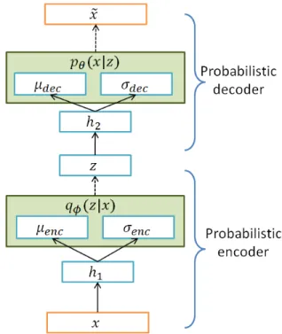
Fig. 1 show the architecture of Gaussian VBAE probabilistic encoder and decoder.

After determining which approximate distribution that we will use to model latent variable z (in this case Gaussian dis- tribution), we can rewrite Eq. 3:

L(θ, φ; x

⁽ⁱ⁾

) = 1

2

J

X

j=1

(1 + log((σ

⁽ⁱ⁾_{enc j}

)

²

) − (µ

⁽ⁱ⁾_{enc j}

)

²

− (σ

⁽ⁱ⁾_{enc j}

)

²

)

+ 1 L

L

X

l=1





 − log σ

^(i,l)_dec

√

2π

−

x

⁽ⁱ⁾

− µ

^(i,l)_dec

2

2σ

^(i,l)_dec²





 . (6) To optimize Eq. 6 w.r.t. probabilistic encoder and decoder

Fig. 1. For generative modelling acoustic features, VBAE uses a Gaussian probabilistic encoder and decoder because the speech features represented by continuous real number. In a probabilistic encoder, we conditionally sample z ∼ q

φ

(z|x) from Gaussian distribution with µ

_enc

and σ

_enc

. The z value passed through probabilistic decoder, and we conditionally sample ˜ x ∼ p

θ

(x|z) from Gaussian distribution with µ

_dec

and σ

_dec

.

parameters, we can use a stochastic gradient method, such

as SGD, Adagrad [18] and Adadelta [19]. In practice, our

experiment use Adagrad for optimizing the VBAE parame-

ters. After several iterations and when marginal log likeli-

hood log p(x) has converged or stabilized, we can use either

the latent variable z from q(z|x) which conditionally sampled from µ

_enc

and σ

enc

as features for a classifier or integrating the entire probabilistic encoder with pretrained parameter and add another DNN with softmax layer on the top of µ

_enc

and σ

enc

. Fig. 2 illustrates how we constructed a discriminative DNN using VBAE’s pretrained probabilistic encoder for ex- tracting latent variable and end-to-end fine-tuning from the negative log-likelihood loss function from the softmax layer.

This stage which is usually called as discriminative finetun- ing, is generally done for classification tasks by several un- supervised pretraining algorithms such as RBM and SDAE.

Fig. 2. We constructed discriminative DNN to output acoustic state probability by removing the probabilistic decoder from VBAE and put randomly initialized hidden and softmax lay- ers. µ

_enc

and σ

enc

are connected into randomly initialized hidden layer with softmax layer on the top of the neural net- work and optimized for acoustic modelling task

5. EXPERIMENTAL SETUP 5.1. Dataset

All the phoneme recognition experiments were performed on the TIMIT corpus dataset

¹

. All the SA records were removed from the experiment. The training set contains 3696 sentences from 462 speakers. Development set was taken from another 50 sets of speakers. Evaluation was done by evaluating our model into core test set that consisted of 192 sentences from 24 different speakers.

1

http://www.ldc.upenn.edu/Catalog/CatalogEntry.jsp?catalogId=LDC93S1

5.2. Front-End

In this experiment, we used speaker adapted fMLLR fea- tures to represent speech signals, which were obtained using a GMM-HMM model built by Kaldi [20] s5 TIMIT recipe for tri3 scenario. Every acoustic frame was represented by 40 features. We used five context windows expanded to the left and right. We combined 11 consecutive acoustic frames combined 440 features per time frame. With the tri3 scenario, the acoustic model states consisted of 1946 tied triphone states, and for decoding we used the phoneme bigram lan- guage model, which was estimated from the training set for decoding purposes.

5.3. Baseline Systems 5.3.1. RBM

Our RBM experiments were done using the KaldiPDNN toolkit [21, 22]. For a baseline RBM experiment, we used a Gaussian-Bernoulli RBM to model our continuous data features from the input layer. Then we stacked multiple Bernoulli-Bernoulli RBM on top of the previous hidden layer and pretrained the layers one by one from the bottom to the top. We used four hidden layers, each of which contains 1024 hidden units. In the end, we put a softmax layer with 1946 units to represent class probability and fine-tuned it using negative log-likelihood cost function.

5.3.2. SDAE

Our SDAE experiments were done using the KaldiPDNN toolkit. For our baseline SDAE experiment, we use tanh nonlinearity to reconstruct input from the hidden layer. We use four hidden layers, each of which contains 1024 hidden units, which is same as the baseline RBM number of hidden layers and unit size. In the end, we put a softmax layer with 1946 units represent class probability and fine-tuned it using negative log-likelihood cost function.

5.3.3. DNN-ReLU + Dropout

In this baseline experiment, we used supervised DNN with rectifier linear activation function and dropout regularization [23]. Indentical as before, we also constructed four hidden layers with rectifier linear activation function with 1024 units for each layer. We tried several dropout probabilities for each layer between 0.2 and 0.5 and selected the best model from development set for the baseline DNN-ReLU+Dropout.

5.4. VBAE-DNN Experiment

For the VBAE experiment, we first built two layers of 1024

hidden units for modelling our probabilistic encoder and 2

layer of 1024 hidden unit for modelling our probabilistic de-

coder. In this experiment, we tried several different numbers

of latent variables within 64, 128, and 256 with L = 1 for each datapoint.

After the generative model training was finished, we used the pretrained probabilistic encoder parameter and projected the unit mean and unit diagonal covariance into one hidden layer and put softmax layer on the top. In the end, we have four hidden layers with 1024-1024-[128,256,512]-1024 units for VBAE-DNN. We also compared two different scenarios, (1) without using dropout, (2) use dropout only at last hidden layer layer before softmax layer. For the second scenario, we used dropout probability 0.25 for the last hidden layer.

6. EXPERIMENT RESULTS

Table 1 compares the performances from various models in terms of phoneme error rates (PER (%)) on the TIMIT core test set. First, the RBM baseline result was 21.1% PER and the SDAE baseline result was 21.6% PER. We also experi- mented on standard DNN ReLU + dropout and trained it with- out unsupervised pretraining and the result was 20.4% PER.

Next we performed an experiment described in section 4 and varied the number of latent variables. The best per- formance for VBAE without dropout regularization was ob- tained both by 64 and 128 latent variables with 20.6% PER.

For the second scenario, by using dropout on the last hidden layer, we improved the recognition performance for both the VBAE with 64 and 128 latent variables to 19.8% PER.

Table 1. Comparison of all experiments in terms of phoneme error rates (PER) on TIMIT core test set

Model Test PER (%)

RBM 21.1

SDAE 21.6

DNN-ReLU+DO 20.4

VBAE (256-latent) 20.9

VBAE (128-latent) 20.6

VBAE (64-latent) 20.6

VBAE+DO (256-latent) 20.0 VBAE+DO (128-latent) 19.8 VBAE+DO (64-latent) 19.8

7. CONCLUSION

This paper explored the use of VBAE trained by SGVB al- gorithm for generative pretraining deep neural networks. Our results reveal that pretrained parameters from a probabilistic encoder of VBAE can produce a better results in comparison with another generative pretraining algorithms with similar neural network configurations. The best accuracy was ob- tained by 64 and 128 Gaussian latent variable VBAE models with 20.6% PER, and we achieved 19.8 % PER with dropout regularization.

In the future, we will further investigate the use of SGVB in various different NN architecture such as Convolutional Neural Network (CNN) and Recurrent Neural Network (RNN) to improve ASR performance. The possibility to utilize SGVB as a feature generator for GMM acoustic model will also be explored. Furthermore, we would be interested to investigate the robustness of this approach for low resources problems in speech recognition.

8. ACKNOWLEDGEMENT

Part of this work was supported by the Commissioned Re- search of National Institute of Information and Communica- tions Technology (NICT) Japan, Microsoft CORE 10 Project, and JSPS KAKENHI Grant Number 26870371. The authors also thank Fasilkom UI High Performance Computing Re- search Group for providing the computational resources.

9. REFERENCES

[1] Lawrence R Rabiner, “A tutorial on hidden markov models and selected applications in speech recognition,”

Proc. of the IEEE, vol. 77, no. 2, pp. 257–286, 1989.

[2] Douglas A Reynolds and Richard C Rose, “Robust text- independent speaker identification using Gaussian mix- ture speaker models,” IEEE Trans. on Audio Processing, vol. 3, no. 1, pp. 72–83, 1995.

[3] G. Hinton, Li Deng, Dong Yu, G.E. Dahl, A. Mohamed, N. Jaitly, A. Senior, V. Vanhoucke, P. Nguyen, T.N.

Sainath, and B. Kingsbury, “Deep neural networks for acoustic modeling in speech recognition: The shared views of four research groups,” Signal Processing Mag- azine, IEEE, vol. 29, no. 6, pp. 82–97, Nov 2012.

[4] Li Deng, Jinyu Li, Jui-Ting Huang, Kaisheng Yao, Dong Yu, Frank Seide, Michael Seltzer, Geoff Zweig, Xiaodong He, Jason Williams, Yifan Gong, and Alex Acero, “Recent advances in deep learning for speech research at microsoft,” in Proc. of ICASSP, 2013, pp.

8604–8608.

[5] Abdel-rahman Mohamed, Geoffrey Hinton, and Gerald Penn, “Understanding how deep belief networks per- form acoustic modelling,” in Proc. of ICASSP, 2012, pp. 4273–4276.

[6] Geoffrey E Hinton, Simon Osindero, and Yee-Whye Teh, “A fast learning algorithm for deep belief nets,”

Neural computation, vol. 18, no. 7, pp. 1527–1554, 2006.

[7] Ruslan Salakhutdinov and Geoffrey E Hinton, “Deep boltzmann machines,” in Proc. of International Confer- ence on Artificial Intelligence and Statistics, 2009, pp.

448–455.

[8] Pascal Vincent, Hugo Larochelle, Isabelle Lajoie, Yoshua Bengio, and Pierre-Antoine Manzagol,

“Stacked denoising autoencoders: Learning useful representations in a deep network with a local denoising criterion,” The Journal of Machine Learning Research, vol. 11, pp. 3371–3408, 2010.

[9] Yoshua Bengio, Aaron Courville, and Pierre Vincent,

“Representation learning: A review and new perspec- tives,” IEEE Transactions on Pattern Analysis and Ma- chine Intelligence, vol. 35, no. 8, pp. 1798–1828, 2013.

[10] Diederik P Kingma and Max Welling, “Auto-encoding variational Bayes,” in Proc of the International Con- ference on Learning Representations, Banff, Canada, 2014.

[11] Fabio Valente and Christian Wellekens, “Variational bayesian GMM for speech recognition,” in Proc. of EU- ROSPEECH, 2003, pp. 441–444.

[12] Shinji Watanabe, Yasuhiro Minami, Atsushi Nakamura, and Naonori Ueda, “Variational bayesian estimation and clustering for speech recognition,” Speech and Audio Processing, IEEE Transactions on, vol. 12, no. 4, pp.

365–381, 2004.

[13] Shinji Watanabe and Jen-Tzung Chien, Bayesian Speech and Language Processing, Cambridge University Press, 2015.

[14] Alex Graves, “Practical variational inference for neural networks,” in Proc. of Advances in Neural Information Processing Systems, 2011, pp. 2348–2356.

[15] Jorma Rissanen, “Modeling by shortest data descrip- tion,” Automatica, vol. 14, no. 5, pp. 465–471, 1978.

[16] Tejas D Kulkarni, Will Whitney, Pushmeet Kohli, and Joshua B Tenenbaum, “Deep convolutional inverse graphics network,” arXiv preprint arXiv:1503.03167, 2015.

[17] Diederik P Kingma, Shakir Mohamed, Danilo Jimenez Rezende, and Max Welling, “Semi-supervised learn- ing with deep generative models,” in Proc. of Advances in Neural Information Processing Systems, 2014, pp.

3581–3589.

[18] John Duchi, Elad Hazan, and Yoram Singer, “Adaptive subgradient methods for online learning and stochastic optimization,” The Journal of Machine Learning Re- search, vol. 12, pp. 2121–2159, 2011.

[19] Matthew D Zeiler, “ADADELTA: An adaptive learning rate method,” arXiv preprint arXiv:1212.5701, 2012.

[20] Daniel Povey, Arnab Ghoshal, Gilles Boulianne, Lukas Burget, Ondrej Glembek, Nagendra Goel, Mirko Han- nemann, Petr Motlicek, Yanmin Qian, Petr Schwarz, Jan Silovsky, Georg Stemmer, and Karel Vesely, “The Kaldi speech recognition toolkit,” in Proc. of IEEE ASRU, 2011.

[21] Yajie Miao, “Kaldi+PDNN: Building DNN-based ASR systems with kaldi and PDNN,” CoRR, 2014.

[22] James Bergstra, Olivier Breuleux, Fr´ed´eric Bastien, Pas- cal Lamblin, Razvan Pascanu, Guillaume Desjardins, Joseph Turian, David Warde-Farley, and Yoshua Ben- gio, “Theano: A cpu and gpu math compiler in python,”

.

[23] Nitish Srivastava, Geoffrey Hinton, Alex Krizhevsky, Ilya Sutskever, and Ruslan Salakhutdinov, “Dropout:

A simple way to prevent neural networks from overfit- ting,” The Journal of Machine Learning Research, vol.

15, no. 1, pp. 1929–1958, 2014.