Similar Subsequence Retrieval from Two Time Series Data Using Homology Search
Takuma Nishii∗,Tomoyuki Hiroyasu†,Masato Yoshimi‡, Mitsunori Miki§ and Hisatake Yokouchi¶
∗Graduate School of Engineering, Doshisha University, Kyoto, Japan Email: [email protected]
†Department of Life and Medical Sciences, Doshisha University, Kyoto, Japan Email: [email protected]
‡Department of Science and Engineering, Doshisha University, Kyoto, Japan Email: [email protected]
§Department of Science and Engineering, Doshisha University, Kyoto, Japan Email: [email protected]
¶Department of Life and Medical Sciences, Doshisha University, Kyoto, Japan Email: [email protected]
Abstract—We propose a method for extracting the most similar subsequences from two time series data by quantizing them and performing a homology search. The homology searches, such as BLAST and SW, are string search algorithms. Therefore, time series data should be quantized. SAX and EIAD were applied as quantization methods, and their effectiveness was examined by experiment. According to the experiments, time series data sets were classified into four types of time series data set, and we discuss the characteristics of SAX and EIAD.
Index Terms—Time Series Data, Smith-Waterman Algorithm, Homology Search, Similarity Search, Requantization
I. INTRODUCTION
Recently, new medical imaging techniques that can obtain biological information, such as functional magnetic resonance imaging (fMRI), optical topography, etc., have come into widespread use. Analysis of the data obtained by these methods will be helpful in investigating brain function. If we can in- vestigate the function of the brain, we can visualize a human’s image in the brain and apply it into various devices. Optical topography measures changes in blood flow and visualizes brain function. For example, this method can be used to visualize the regions of the brain activated when singing or watching TV. We can understand which parts of the brain operate the feelings of happy by analyzing the experimental data that a man ”listening music happily” and ”eating lunch happily”. However, optical topography outputs more than 300 time series data in a single experiment. With such large amounts of data, it is difficult to determine on which data to focus. The time series data from optical topography require searching to allow time warping. It is good way for the analysts to reduce task to search for similar parts allowing time warping automatically from multiple time series data. Here, we propose a method for extracting the most similar subsequences from two time series data by quantizing the data and performing a homology search.
Active Search is a method of detecting objective patterns from large data that achieves high speed and accuracy and
is used for visual or acoustic patterns. Time series Active Search (TAS) [1] and DTW (Dynamic Time Warping) [2]
are examples of Active Search algorithms. Interval-Free Time series Active Search (RIFTAS) [3] and Interval-Free Continu- ous Dynamic Programming (RIFCDP) [4] are algorithms for searching similar parts of two time series data. These algo- rithms repeat TAS or DTW by changing the window size and subsequences. However, these algorithms incur tremendous calculation costs for dealing with actual data. Toyoda proposed a function to recognize the similarity between subsequences for data streams using DTW [5]. This function is efficient and works well but requires a threshold value. Keogh proposed a method to find frequently occurring patterns called ”motifs” in time series data [6]. This method cannot be applied to more than two time series data. Discrete Fourier Transform (DFT) and Cross Correlation Function [7] cannot compare similarity allowing time warping. Thus, there are several ways to search for similar parts of multiple time series data allowing time warping. However, processing of multiple time series data requires large computational resources. Thus, It is effective to use parallelized algorithms to process large and multiple time series data quickly. In addition, it is better to use the algorithm in the field that already has many parallelized algorithms.
In this paper, we propose a method for extracting the most similar subsequences of two time series data by ho- mology search that the program library has many parallelized algorithms. It is necessary to quantize time series data as strings because homology search algorithms are string search algorithms. SAX and EIAD are typical algorithms used to quantize time series data. Here, we propose a method for extracting the most similar subsequences of two time series data by quantizing the data and then using homology search to determine similar regions between the two sequences. SAX and EIAD were applied and the results of these methods were compared by experiment.
mds March 15, 2010
㻌㻌㻌㻌㻭㻌㻌㻭㻌㻌
㻮㻌㻌㻌㻌㻌㻌㻌㻌㻌㻌㻮㻌㻌㻌㻌㻌㻌㻌㻌㻌㻌㻮㻌 㻌㻌㻌㻌㻌㻌㻌㻌㻌㻌㻌㻌㻌㻌㻌㻌㻌㻌㻯㻌㻌㻌㻯
㻌㻌㻌㻌㻭㻌㻌㻌㻌㻌㻌㻌㻌㻌㻌㻌㻌㻌㻌㻌㻌㻌㻭㻌㻌㻭㻌㻌 㻌㻌㻮㻌㻌㻌㻌㻌㻌㻌㻌㻌㻌㻮㻌 㻌㻌㻌㻌㻌㻌㻌㻌㻌㻌㻯㻌㻌㻌㻯
㻮㻭㻭㻮㻯㻯㻮
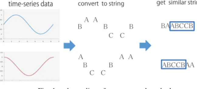
㻭㻮㻯㻯㻮㻭㻭 convert to string get similar string time-series data
Fig. 1. the outline of our proposed method
II. METHOD FOR EXTRACTION OF SIMILAR SUBSEQUENCES FROM TWO TIME SERIES DATA BY
HOMOLOGY SEARCH
A. Concept of the proposed method
In this paper, we propose a method for extracting the most similar subsequences from two time series data by quantizing time series data and performing a homology search. Fig.1 shows the outline of our proposed method.
First, we quantize the time series data. For example, the upper and lower time series data sets in Fig.1 are converted to”BAABCCB” and ”ABCCBAA,” respectively. There are several methods for quantizing the data. Here, we focus on SAX and Equal Intervals Area Division (EIAD) as quan- tizing methods. Second, we apply homology search to the quantized time series data. The homology search algorithm is an algorithm for performing sequence alignment. Finally, this algorithm can extract ”ABCCB” as a similar section of
”BAABCCB” and ”ABCCBAA”. In this way, we can extract part of time series data with similarity by quantizing the time series data and extracting similar sections. In addition, we applied the Smith-Waterman (SW) algorithm for homology search. The SW algorithm, described in the following section, can perform time warping search by the gap parameter.
B. Quantization of time series data
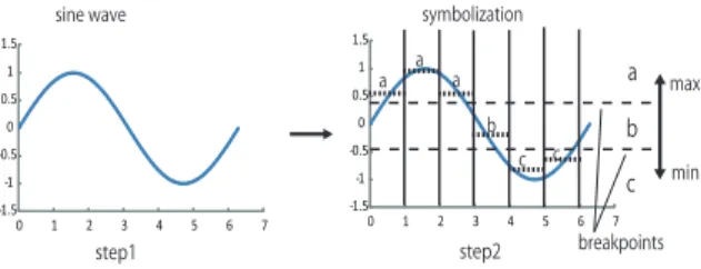
This algorithm needs to provide the relation between numerical value and character. For example, a time series T = {1.0,1.5,−0.5} is symbolized as ”BAC”. To perform this transformation, breakpoints should be defined. SAX and EIAD are typical algorithms used to quantize time series data. In SAX, the time series data histogram is assumed to have a normal distribution. On the other hand, in EIAD, the time series data histogram is assumed to have a uniform distribution. The number of breakpoints is very important and this parameter affects the results of similar sequence extraction.
1) SAX(Symbolic Aggregation Approximation): SAX is a method proposed by Keogh to represent time series data [8]. This algorithm assumes that time series data have a normal distribution and symbolizes the time series data. As SAX assumes a Gaussian distribution, time series data must be normalized before converting to a string. Standardization means to convert the averages of certain data to 0 and standard deviation to 1. For example, a time seriesT =t1, . . . , tM will be converted toT= (t1−µ)/σ, . . . ,(tM−µ)/σ, whereµand σare the average and standard deviation of T, respectively.
Fig.2 illustrates the concept of normalization and sym- bolization of SAX. In step 1 of Fig.2, we normalize the time series data. In step 2, we symbolize the time series data to a string. Normalized subsequences have a highly normal distribution. Therefore, we can simply determine the
”breakpoints” that will produce equal-sized areas under the normal curve [8]. Breakpoints are a sorted list of numbers B = (β1, . . . , βn). These breakpoints may be determined by referencing a statistical table. Table.I gives the breakpoints for values of α from 2 to 7. In Fig.2, data that are below the smallest breakpoint are mapped as the symbol ”c”. Data greater than or equal to the smallest breakpoint and less than the second smallest breakpoint are mapped as the symbol ”b”.
Other data are mapped as the symbol ”a”. Consequently, the time series data in Fig.2 are mapped as ”aaabcc”.
-1.5 -1 -0.5 0 0.5 1 1.5
0 1 2 3 4 5 6 7
normalization
-1.5 -1 -0.5 0 0.5 1 1.5
0 1 2 3 4 5 6 7
b
a a a
c c
breakpoints a b c symbolization
step2
step1 normal distribution curve
33%
33%
33%
Fig. 2. the concept of Symbolic Aggregation approXimation
TABLE I
BREAKPOINTS THAT DIVIDE A NORMAL DISTRIBUTIONIN AN ARBITRARY NUMBER FROM2TO7OF EQUIPROBABLE REGIONS
α 2 3 4 5 6 7 8
β1 0 -0.43 -0.67 -0.84 -0.97 -1.07 -1.15
β2 0.43 0 -0.25 -0.43 -0.57 -0.67
β3 0.67 0.25 0 -0.18 -0.32
β4 0.84 0.43 0.18 0 β5 0.97 0.57 0.32
β6 1.07 0.67
β7 1.15
2) EIAD(Equal Intervals Area Division): The EIAD as- sumes a uniform distribution of the time series data histogram.
Breakpoints divide the minimum and maximum values of the time series into equal areas. This method has different breakpoints and it is not necessary to standardize the time series data. Fig.3 shows the concept of the EIAD.
For example, time series data with maximum and minimum values of 1.0 and -1.0 would be symbolized as three characters with the breakpoints (0.34, -0.34). The width of the area becomes 0.68. The following equations show how to determine the width of the area
w=|M AX−M IN | ÷N U M (1) breakpoints=M AX−W ×N(1≤n≤N U M−1) (2) where MAX and MIN are the maximum and minimum values of time series data, respectively. W is the width of the area, and NUM is the number of characters.
-1.5 -1 -0.5 0 0.5 1 1.5
0 1 2 3 4 5 6 7
-1.5 -1 -0.5 0 0.5 1 1.5
0 1 2 3 4 5 6 7
b
a a a
c c
breakpoints a b c sine wave
step1
symbolization
step2
max min
Fig. 3. the concept of Equal Intervals Area Division
III. HOMOLOGY SEARCH AND THESMITH-WATERMAN
ALGORITHM
Homology search is performed by string search algorithms to examine the homology of the living things. These algorithms are used to determine regions of similarity between two or more nucleotide or protein sequences. Nucleotide and protein sequences are normally very long, and searching them requires huge computational resources. Use of parallelized algorithms is a very effective means to reduce computational time. As it is necessary to deal with long sequences in bioinformatics, many parallelized program libraries for homology searching have been developed. Use of these parallelized algorithms allows searching of time series data quickly.
SW, BLAST, and FASTA are well-known homology search algorithms. SW focuses on accuracy, while FASTA and BLAST focus on speed. Here, we adopted SW because the time series data set used for accuracy validation was limited.
The SW algorithm is used for local sequence alignment.
SW is a dynamic programming algorithm and compares seg- ments of all possible lengths and optimizes the similarity measure.The similarity measure is evaluated by scoring a two- dimensional matrix. There is one column for each character in sequence A and one row for each character in sequence B in this matrix. If we are aligning sequences of sizes n and m, the order of this algorithm is O(mn). The SW algorithm allows time warping search by the gap parameter.
A. Parameters of score
This algorithm needs scoring, match, mismatch, and gap penalty parameters. Gap means insertion or deletion of spaces.
The result will be affected by changes in these parameters.
The parameters match = 1, mismatch = -1, and gap = -1 are standard settings. The results for match = 1, mismatch = -1, and gap = -0.5 will have more spaces than the standard setting.
In addition, the results for match = 1, mismatch = -2, and gap
= -2 will have higher similarity than the former but the result will be shorter in length. The best parameters will be changed according to the required similarity. Here, we used the standard setting: match = 1, mismatch = -1, and gap = -1.
B. Algorithm
The process of obtaining the optimum local alignment is illustrated as follows. First, we initialize two-dimensional matrix then score a match or a mismatch of each cell. If we finished scoring untill the end of matrix, we start backtracing from maximum cell score. Backtracing means to obtain the
optimum local alignment by walking back to the zero cell score from the maximum cell score.
Fig.4 shows the SW algorithm. Fig.6, Fig.7, Fig.8, and Fig.9 show the process of obtaining the optimum local alignment between ”BBC” and ”CBC”.
step1 Initializing two-dimensional matrix(Fig.6)
step2 Scoring a match or a mismatch of each cell(Fig.7) step3 Scoring until the end of the matrix(Fig.8)
step4 Backtracing from maximum cell score(Fig.9)
Fig. 4. Smith-Waterman algorithm
Equations (3) and (4) show formulas for calculating the scores for aligned characters in the matrix. Each cell s score is calculated from the left, right, and upper cells’ scores, and match or mismatch of aligned characters. For example, the (1,1) cell s score will be calculated by equation (4) because of the alignment shows a mismatch (Fig.7), SW(1,1) = max{SW(0,1) - 1, SW(0,0) - 1, SW(1,0) - 1, 0}= 0. The (1,2) cell s score will be calculated by (3) because the alignment shows a match (Fig. 6), SW(1,1) =max{SW(0,1) - 1, SW(0,0) - 1, SW(1,0) - 1, 0} = 0. If the calculated score is 0, the cell is assigned a score of 0.
To obtain the optimum local alignment, we start with the highest score in the matrix and walk back to the zero score.
Each cell has the previously calculated path. In Fig.8, the highest score corresponds to the cell in position (3,3). The walk back corresponds to (3,3), (2,2), (1,1). We reiterate the process until we reach a matrix cell with zero score or the score in position (0,0). Once we have finished, we reconstruct the alignment. The upper character of the (3,3) cell is ”B” and the left character is ”C”. The upper character of the (2,2) cell is ”B” and the left is ”B”. Then, the optimum local alignment of ”BBC” is ”BC” and that of ”CBC” is ”BC”. Fig.5 shows the example of SW algorithm alignment.
[h]SW(y, x) =max
SW(y−1, x−1) +match SW(y−1, x) +gap SW(y, x−1) +gap 0
(3)
[h]SW(y, x) =max
SW(y−1, x−1) +mismatch SW(y−1, x) +gap
SW(y, x−1) +gap 0
(4)
IV. EXPERIMENTALEVALUATION
A. Goal of the experiment
We applied our proposed method to several types of data set to compare the similar parts of time series data using SAX and EIAD and to confirm the types of data to which use our method is appropriate.
”PELICAN” →”ELICAN”
”PAWHEAE”→ ”AW HE”
”COELACANTH”→ ”ELACAN”
”HEAGAWGHEE”→ ”AWGHE”
Fig. 5. Example of SW algorithm alignment
x |y _ C B C
_ 0 0 0 0
B 0
B 0
C 0
Fig. 6. Initializing two-dimensional matrix
x |y _ C B C
_ 0 0 0 0
B 0
B 0
C 0
(1,1)
Fig. 7. Scoring a match or a mismatch of each cell
x |y _ C B C
_ 0 0 0 0
B 0 0 1 0
B 0 0 1 0
C 0 1 0 2
Fig. 8. Scoring until the end of the matrix
x |y _ C B C
_ 0 0 0 0
B 0 0 1 0
B 0 0 1 0
C 0 1 0 2(max)
Fig. 9. Backtracing from maximum cell score
B. Data set
We used the time series data set prepared by UCR [9].
This data set includes some type of numerical time series data in multiple classes. In this experiment, we assumed that two time series data in the same class were similar. We extracted the whole time series data belonging to the same class as the similar part. Figures 10 to 17 have two time series data and the similar part is shown in black, with the rest shown in gray.
For the sake of simplicity, the strings of each time series data are not shown. The figures of SAX are different from those of EIAD because the former standardizes the time series data.
We used 5 breakpoints based on the results of preliminary experiments. We set the parameters as follows: match = 1, mismatch = -1, and gap = -1.
C. Evaluation method
The similar parts of SAX and those of EIAD are different.
To compare the two different subsequences, the length and coincidence of the sequences were examined. To examine the coincidence, DTW (Dynamic Time Warping) distance was performed. DTW is an algorithm for measuring similarity between two sequences, which may vary in time or speed. That is, DTW is a distance measure that allows time warping. For example, similarities in speaking patterns would be detected even if one person is talking slowly and another is speaking more quickly. DTW distance is defined as follows:
DT W(P, Q) =f(np, nq) (5)
f(i, j) =|pi−qj|+min
f(i, j−1) f(i−1, j) f(i−1, j−1)
f(0,0) = 0, f(i,0) =f(0, j) =∞ (i= 1, . . . , npj = 1, . . . , nq)
We can define a margin of error by DTW distance/length. By the margin of error we can judge which way extract better similarity part. This is because low margin of error means high similarity.
TABLE II
DTWDISTANCE OF SIMILAR SUBSEQUENCES IN EACH FIGURE
Figure Name Distance Length Dis/Len
Fig.10 41.6 114 0.36
Fig.11 53.3 118 0.45
Fig.12 32.2 112 0.29
Fig.13 16.3 67 0.24
Fig.14 10.6 63 0.17
Fig.15 23.2 222 0.10
Fig.16 1.1 1 1.09
Fig.17 42.6 4 10.65
D. Experimental results
We tested several types of time series data by SAX and EIAD. Here, four typical data sets are shown. Table.II sum- marizes the results of DTW distance of similar subsequences.
Fig.10 and Fig.11 show the good results of SAX and EIAD.
In this case, two time series data with different phases were used and even each time series data’s phase are shifted, the similar data is properly extracted. Thus, the proposed method can be used to extract similar subsequences from time series data with shifted phases.
Fig.12 and Fig.13 show the good results of EIAD but poor results of SAX. In this case, SAX partially extracted similar subsequences from those expected to be similar. Fig.13 shows
that the breakpoints were not set properly. The similar part appears difficult to extract if the data increase and decrease intermittently on the breakpoints.
Fig.14 and Fig.15 show the poor results of EIAD but good results of SAX. This case had the outliers in the data, which prevented EIAD from extracting similar subsequences.
Fig.16 and Fig.17 show the poor results of SAX and EIAD. Fig.16 had outlier in data, which prevented EIAD from extracting similar subsequences. Fig.17 shows an example in which the scale was changed by normalization. This changed the breakpoints and prevented extraction working properly.
-3 -2 -1 0 1 2 3
1 21 41 61 81 101 121 141
-3 -2 -1 0 1 2 3
1 21 41 61 81 101 121 141
Fig. 10. Leaf all dataset:EIAD
-3 -2 -1 0 1 2 3
1 21 41 61 81 101 121 141
-3 -2 -1 0 1 2 3
1 21 41 61 81 101 121 141
Fig. 11. Leaf all dataset:SAX
-2 -1.5 -1 -0.5 0 0.5 1 1.5 2
1 21 41 61 81 101 121
-2 -1.5 -1 -0.5 0 0.5 1 1.5 2
1 21 41 61 81 101 121
Fig. 12. CBF dataset:EIAD
-2 -1.5 -1 -0.5 0 0.5 1 1.5 2
1 21 41 61 81 101 121
-2 -1.5 -1 -0.5 0 0.5 1 1.5 2
1 21 41 61 81 101 121
Fig. 13. CBF dataset:SAX
-4 -3 -2 -1 0 1 2 3 4
1 2141 61 81101121141161181201221241261
-4 -3 -2 -1 0 1 2 3 4
1 21 4161 81101121141161181201221241261
Fig. 14. Trace dataset:EIAD
-4 -3 -2 -1 0 1 2 3 4
1 2141 61 81101121141161181201221241261
-4 -3 -2 -1 0 1 2 3 4
1 21 4161 81101121141161181201221241261
Fig. 15. Trace dataset:SAX
0 5 10 15 20 25 30 35 40 45 50
1 6 11 16 21 26 31 36 41 46
0 5 10 15 20 25 30 35 40 45 50
1 6 11 16 21 26 31 36 41 46
Fig. 16. Q8Humid dataset:EIAD
-7 -6 -5 -4 -3 -2 -1 0 1 2 3
1 6 11 16 21 26 31 36 41 46
-7 -6 -5 -4 -3 -2 -1 0 1 2 3
1 6 11 16 21 26 31 36 41 46
Fig. 17. Q8Humid dataset:SAX
As shown in Table.II, the margins of error of SAX and EIAD are almost the same. In this experiment, we focused on two factors, the length and error of the derived sequences.
As the errors of the extracted sequences were the same, the sequences with the longer length are better. Here, the four types of time series data set are shown, and SAX and EIAD each have advantages and disadvantages depending on the time series data. If the time series data have no outliers, EIAD is better for extraction because of the longer width of breakpoint area. The converse is true if the time series data have some outliers, and SAX appears to be better for extraction. It is difficult for SAX and EIAD to extract the similar part if the data increase and decrease intermittently on the breakpoints.
Both methods can extract similar subsequences from two time series data of different phase. These results indicate that the proposed method needs prior processing of time series data, such as removing outliers or smoothing. The proposed method can extract similar subsequences from two time series data of different phase by prior processing.
V. CONCLUSIONS ANDFUTUREWORK
In this paper, we proposed a method for extracting the most similar subsequences from two time series data by quantizing the time series data and using homology search. Several good parallel implementations are available for the homology search, such as BLAST and the SW algorithm. When these parallel algorithms are used, the computational time can be reduced.
At the same time, we aim to extract similar parts using partial rather than exact matches. The SW algorithm allows extraction of partial matches by time warping search. However, it is necessary to quantize the time series data because SW is a string search algorithm. In this paper, we compared two quantized algorithms, SAX and EIAD. Both SAX and EIAD were applied in the experiments and the results were evaluated with four types of time series data set. In the first data set, both methods could extract similar subsequences from two time series data of different phase. In the other data sets, we presented cases in which SAX was better than EIAD and others in which EIAD was better than SAX. There were also data sets where neither EIAD nor SAX could find appropriate similar parts.
In future work, the parameters of the SW algorithm and the optimal number of breakpoints should be defined. Pretreatment of the data, such as removing the outliers and smoothing, should be discussed. In this paper, only two time series data sets were described, but more than three data sets should be applied.
REFERENCES
[1] KASHINO Kunio,SMITH Gavin A,MURASE Hiroshi, ”A Quick Search Algorithm for Acoustic Signals Using Histogram Features”, The trans- actions of the Institute of Electronics, Information and Communication Engineers. D-II pp.1365-1373 19990925
[2] SAKURAI Yasushi YOSHIKAWA Masatoshi, ”A Similarity Search Method for Dynamic Time Warping”, Information Processing Society of Japan pp.23-36 20040315
[3] NISHIMURA Takuichi,MIZUNO Michinao,OGI Shinobu,SEKIMOTO Nobuhiro,OKA Ryuichi, ”Same Interval Retrieval from Time-Sequence Data Based on Active Search : Reference Interval-Free Time : Series Active Search (RIFAS)”,The transactions of the Institute of Electronics, Information and Communication Engineers. D-II pp.1826-1837 20010801 [4] ITOH Yoshiaki,KIYAMA Jiro,KOJIMA Hiroshi,SEKI Susumu,OKA Ryuichi ”Reference Interval-free Continuous Dynamic Programming for Spotting Speech Waves by Arbitrary Parts of a Reference Sequence Pattern”, The Institute of Electronics, Information and Communication Engineers pp.1474-1483 19960925
[5] TOYODA Machiko,SAKURAI Yasushi, ICHIKAWA Toshikazu ”Stream Matching based on Dynamic Programming”
[6] Abdullah Mueen, Eamonn Keogh, Qiang Zhu, Sydney Cash, Brandon Westover, ”Exact Discovery of time series Motifs”, SDM 2009: 473-484 [7] KATAYAMA Erika,YAMADA Yoshio,TSUZUKI Shinji ”A Method for Peak Position Estimation of Cross Correlation Functions Using Neural Network”, The Institute of Image Information and Television Engineers pp.21-24 20010302
[8] Lin J, Keogh E, Lonardi S, Chiu B, A Symbolic Representation of time series, with Implications for Streaming Algorithms. In proceedings of the 8th ACM SIGMOD Workshop on Research Issues in Data Mining and Knowledge Discovery.
[9] Eamonn Keogh, Xiaopeng Xi, Li Wei, and Chotirat (Ann) Ratanama- hatana, ”Welcome to the UCR time series Classification/Clustering Page”, http://www.cs.ucr.edu/∼eamonn/time series data/