Partial differential equations

Partial differential equations

Takehito Yokoyama

Department of Physics, Tokyo Institute of Technology, 2-12-1 Ookayama, Meguro-ku, Tokyo 152-8551, Japan

(Dated: January 30, 2014)

PARTIAL DIFFERENTIAL EQUATIONS

Types of partial differential equations are summarized as follows.

∂ ² u

∂t ² = c ² ∂ ² u

∂x ² Wave equation (1)

∂ ² u

∂t ² = c ² ∂ ² u

∂x ² − k ∂u

∂t Wave equation with friction (2)

∂ ² u

∂t ² = c ² ∂ ² u

∂x ² − k ∂u

∂t − hu Transmission line equation (3)

∂ ² u

∂t ² = − b ² ∂ ⁴ u

∂x ⁴ Beam equation. (4)

∂u

∂t = D ∂ ² u

∂x ² Diffusion equation (5)

∂u

∂t = D ∂ ² u

∂x ² − ku Diffusion equation with lateral concentraton loss (6)

∂u

∂t = D ∂ ² u

∂x ² − v ∂u

∂x Diffusion − convection equation (7)

∂u

∂t = D ∂ ² u

∂x ² − u ∂u

∂x Burgers equation. (8)

Note

Some notes on the partial differential equations listed above are presented. Some transformations can simplify the equations:

In the transmission line equation, this transformation eliminates the u t term

u = e

^kt/2 w. (9)

In the diffusion equation with lateral concentraton loss, this transformation reduces it to the simple diffusion equation

u = e

^kt w. (10)

In the diffusion-convection equation, this transformation reduces it to the simple diffusion equation

u = e

^v[x

^vt/2]/2D w. (11)

The solution of the Burgers equation can be constructed by the following transformation where ψ obeys the simple diffusion equation :

u = − 2D ∂

∂x ln ψ. (12)

This transformation is called the Hopf-Cole transformation. The solution of the initial value problem of the Burgers equation thus reads [u(x, 0) = f (x)]

u = − 2D ∂

∂x ln 1

2 √ πDt

Z

−∞

exp

− (x − y) ²

4Dt + 1

2D Z y

0

f (z)dz

dy

. (13)

2

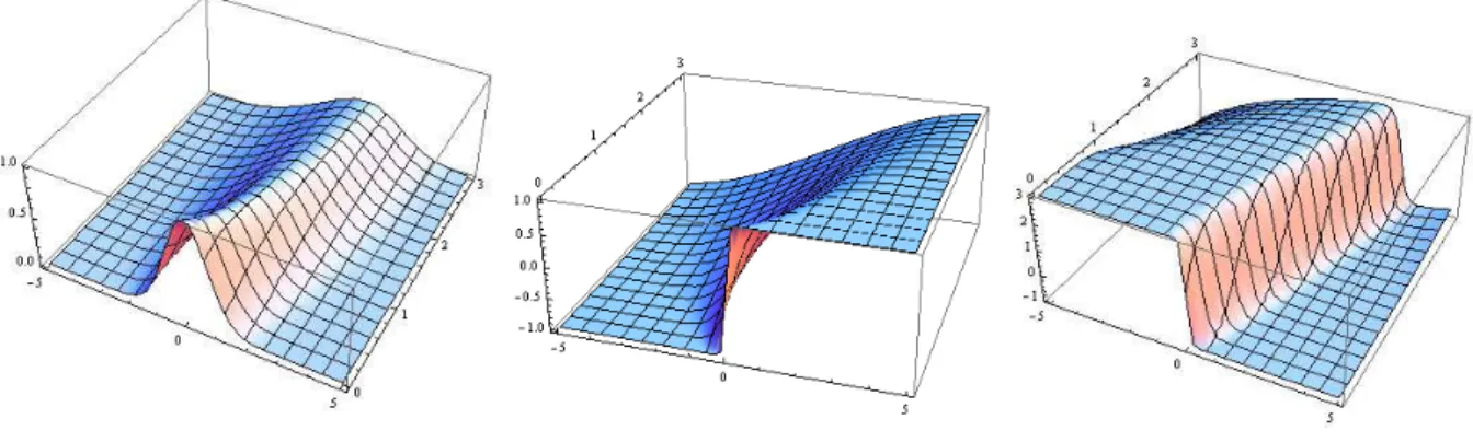
FIG. 1: Plots of u(x, t). Left: u(x, 0) = e

. Middle: u(x, 0) = tanh(10x). Right: u(x, 0) = 1 − 2 tanh(10x).

Typical solutions of the Burgers equation are shown in Fig. 1. Interestingly, we see a shock wave solution in the right panel. Intuitively, this is because the velocity of the wave is given by u. Thus, the larger the magnitude of u, the faster the wave travels. This interpretation is consistent with Fig. 1.

Derivation of the beam equation

Consider a beam along x-axis. We have two assumptions: No cross-sectional deformation:

ε _yy = ε _zz = ε _yz = 0. (14)

and Bernoulli-Euler assumption (Bernoulli-Euler Beam):

ε xy = ε xz = 0. (15)

Here, the strain tensor ε ij is defined as

ε ij = 1 2

∂u i

∂x j

+ ∂u j

∂x i

. (16)

u i is the displacement vector. The diagonal elements represent extensional strain while the off-diagonal elements denote shearing strain.

Let u(x) a displacement along the x-axis, w(x) a deflection along y-axis, and θ(x)( ≪ 1) a slope of the beam. Then, we have

u x = u − y sin θ ≃ u − yθ, u y = w + y(1 − cos θ) ≃ w. (17) Since ε xy = 0, we obtain

θ = dw

dx . (18)

Therefore, we arrive at

ε xx = du

dx − y d ² w

dx ² . (19)

According to the Hooke’s law, we obtain the normal stress of the beam:

σ xx = Eε xx = E du

dx − y d ² w dx ²

(20) where E is the Young’s modulus. The bending moment of the beam M can be calculated as

M = Z

A

yσ xx dA = EJ y

du

dx − EI d ² w

dx ² . (21)

3 Here, dA is the infinitesimal section area. J y and I denote the first sectional moment and the sectional moment of inertia, respectively:

J y = Z

A

ydA, I = Z

A

y ² dA. (22)

If the x-axis goes through a centroid of the section, we have J y = 0.

Now, consider the equation of motion of the beam:

ρA ∂ ² w

∂t ² = ∂V

∂x + p (23)

where ρ is the density, p is the external force, V is the shear force. The equilibrium equation of moments reads

∂M

∂x = V. (24)

Thus, we finally obtain the beam equation:

ρA ∂ ² w

∂t ² = − EI ∂ ⁴ w

∂x ⁴ + p. (25)

In the presence of viscous drag, the normal stress of the beam is given by σ xx = Eyκ + ηy ∂κ

∂t . (26)

Here, η is the viscosity coefficient, and κ represents the curvature of the beam, κ = − ^∂ ∂x

^w

. The equation of motion of the beam then becomes

ρA ∂ ² w

∂t ² = − EI ∂ ⁴ w

∂x ⁴ + − ηI ∂ ⁵ w

∂t∂x ⁴ + p. (27)

Alternatively, the kinetic and potential energies of the beam, K and U , are respectively given by K = 1

2 Z

ρA ∂w

∂t 2

dx, U = 1 2

Z

σ xx ε xx dAdx = 1 2

Z

M κdx = 1 2

Z EI

∂ ² w

∂x ^{2 2}

dx. (28)

Variation of the action with respect to w also gives the beam equation.

OTHER PARTIAL DIFFERENTIAL EQUATIONS

We know the solutions of ^∂u _∂t = L[u] for L[u] = u x and u xx . As a next step, consider the case of L[u] = u xxx :

∂u

∂t = ∂ ³ u

∂x ³ . (29)

The solution for u(x, 0) = f (x) can be obtained by Fourier transforming the equation:

u = Z

−∞

F (x − y, t)f (y)dy, (30) F (x, t) = 1

2π Z

−∞

exp ik ³ t − ikx

dk = (3t)

^1/3 Ai

− x (3t) ^1/3

. (31)

Here, Ai(x) is the Airy function defined as Ai(x) = 1

2π Z

−∞

exp

i k ³ 3 + ikx

dk. (32)

Incorporating uu x and u xxx terms, we arrive at the KdV equation:

∂u

∂t + u ∂u

∂x + ∂ ³ u

∂x ³ = 0. (33)

4

FIG. 2: The solutions of the KdV equation for u(x,0) = 8sech

(0.5x). Time evolution of the wave from upper left to lower right.

This equation has a traveling-wave solution given by u(x − vt) = 3vsech ²

r v

2 (x − vt + c)

(34) where c is a constant.

The KdV equation can describes solitons. See the solutions of the KdV equation in Fig. 2. Solitary waves propagate with independent velocities.

The solution of the following equation can be constructed by u = ψ ² + _∂x ^∂ ψ (dubbed the Miura transformation)

∂u

∂t − 6u ∂u

∂x + ∂ ³ u

∂x ³ = 0 (35)

where ψ satisfies

∂ψ

∂t − 6ψ ² ∂ψ

∂x + ∂ ³ ψ

∂x ³ = 0. (36)

Finally, let us consider the sine-Gordon equation:

∂ ² u

∂t ² = c ² ∂ ² u

∂x ² − sin u. (37)

This equation has a traveling-wave solution of the form u(x − vt). Then, the equation is reduced to u

= 1

c ² − v ² sin u. (38)

The solution is then given by

u(x − vt) = 4 tan

¹

exp

± x − vt

√ c ² − v ²

(39)

for c ² > v ² under the boundary condition cos u → 1 (x → ∞ ). For c ² = v ² , the solution is trivial. For c ² < v ² , the

equation is reduced to that of a simple pendulum, which can be written with elliptic functions as we saw in another

note.