JAXA Research and Development Report
February 2017
Japan Aerospace Exploration Agency
MID-INFRARED VARIABILITY OF ACTIVE GALACTIC
NUCLEI WITH THE
AKARI
AND
WISE
ALL-SKY SURVEYS
ABSTRACT
Westudied mid-infrared(mid-IR)variability ofAGNsystematically combiningtwo all-sky survey catalogs releasedbyAKARIand Wide-fieldInfraredSurvey Explorer(WISE). Becausethetwo sur-veys areseparated by ∼4 years, ourstudiesare sensitiveto variationsof time scalesofa fewyears. We started with the list of AGN selectedby Matsuta et al. (2012) from the cross-identification of
Swift/BATand AKARIcatalogs. Thelist wasfurther correlatedwiththe WISEcatalog to selecta totalof71AGN,whichwereusedforthepresentstudies. Wecomparedsourcefluxesin theAKARI
S9W(9µm)andWISEW3(12µm)bandsandintheAKARIL18W(18µm)andWISEW4(22µm) bandscarefullycorrectingforthebanddifferencesandconsideringthesystematiceffects. Wedetected significantflux changesfrom3sources,twoblazars(3C273,3C345)andaradiogalaxy(3C445),in the mid-IRbands. This isthefirst detectionofmid-IR variabilityfrom 3C445,whichmay be orig-inatedfrom thejets. Wealso analyzedaveragesamplevariabilityfordifferentAGNtypesexcluding these3variablesources. WedetectedsignificantvariationsfromSeyfert1intheS9W-W3bandwith 95% confidence limit;theaveragefractionalvariability reached 13%(6–18%). Twoorigins are con-ceivableforthevariability: thedustytorusandthejets. Ifsuchvariabilityoriginatesfromthetorus, thedust distributioninthetorus shouldbe verynarrow, anditsradial extentmaybe muchsmaller thanthedistancetotheAGN.Alternatively,thevariabilitymayresultfromthejetsconsideredtobe presentin Seyfert1 galaxies.
Subject headings:activegalacticnuclei,infraredsources,X-raysources
1. INTRODUCTION
Activegalacticnuclei(AGN)produceenormousamountofenergyfromthecentralcompactregionharboringasuper massiveblackhole. MassaccretionontotheblackholessustainthelargeluminosityofAGN,althoughthegeometry andemissionmechanismin thenuclearregionarenotwellunderstoodyet. LuminosityvariationsofAGN,whichare theircommonproperties,conveyprecious informationto probethenuclearregionunlessotherwisedifficulttoobtain (e.g. Ulrichetal.1997).
Timevariationsmayhavedifferentproperties indifferentwavebandsdependingontheemissionmechanisms. The UV/optical continuumvariabilitytends tobe correlatedwith that ofX-rayswith littletimedelay. This meansthat theUV/opticalemissionmaybe duetothereprocessing oftheX-rayemissionfromthecentral source. Somemodels explainthattheUV/opticalemissionisproducedbyanopticallythickmedium(i.e.,accretiondisk)irradiatedbythe variable centralX-ray source(Haardt&Maraschi1993). Infrared (IR)variationshave smalleramplitudeand longer timescalethanthoseinUV/opticalbands(Neugebaueretal.1989;Huntetal.1994). Innear-IRband,variationswith timescalesontheorderofyearsareseenin theradio-loudquasars,whoseamplitudeislessthan1mag. Variationsof Seyfert1s andquasarsof226sampleswerestudiedin near-IRforatime scaleof afewyears (Enyaetal.2002a,b,c). Theyarguedthat near-IRvariabilityof theradio-quietAGNisconsistent witha simpledust reverberation,butthat of radio-loudAGNmay require anon-thermalvariable component. Ontheotherhand,in themid-IRband,there is no strong andrapid variation thanthat of X-ray and UV/optical emissionsexcept forblazars. A few sources show variability on timescale of a year, whose average amplitude reaches ∼10% at 10 µm with a significant time delay compared to variationsofUV/optical continuum(e.g., Clavel et al.1989;Neugebauer &Matthews 1999;Gorjianet al.2004;Koz�lowskietal.2010).
Amongthetimevariationsin variouswavebands, mid-IRvariationscan potentiallyconstrainthegeometryof the dusty torus, becausethey enableusto measure theresponse ofthe torusto changes ofthe direct emissionfrom the nucleus(H¨onig&Kishimoto2011). However, pastobservationsofmid-IRvariabilityofAGNweremademostlyfrom ground, and weremuchfewer thanthose in other wavebands. Thesituation haschangedrecently when theall-sky survey data from space became available including the mid-IR band. Therefore, we studied a long-term variation at mid-IR bands bycombiningthe two all-skysurvey catalogs,theAKARI Point Source Catalogues (AKARI/PSC; Ishiharaetal.2010;Yamamuraetal.2010)andtheWISEAll-SkySourceCatalog(WISE;Wrightetal.2010). AKARI
(Murakami etal.2007)scannedthewholeskytwiceormore duringthe16monthsofthecryogenicmissionphasein
K.Matsuta1,2,4, T.Dotani1,2,P. Gandhi2,3,T.Nakagawa2, K.Enya1,2, H.Matsuhara1,2,S.Takita2,Y.Toba1,2
doi: 10.20637/JAXA-RR-16-010E/0001 * Received November 30, 2016 1
Department of Space and Astronautical Science, The Graduate University for Advanced Studies, 3-1-1 Yoshinodai, Chuo-ku, Sagamihara, Kanagawa 252-5210, Japan
2
Institute of Space and Astronautical Science, Japan Aerospace Exploration Agency, 3-1-1 Yoshinodai, Chuo-ku, Sagamihara, Kanagawa 252-5210, Japan
3
Department of Physics, University of Durham, South Road, Durham DH1 3LE, UK
MID-INFRARED VARIABILITY OF ACTIVE GALACTIC NUCLEI
WITH THE AKARI AND WISE ALL-SKY SURVEYS
ABSTRACT
2006–2007. On the other hand,WISEconducted all-sky surveys with high sensitivity in several mid-IR bands in 2010 about 4 years after AKARI. As we are interested in variability of AGN, we need to pick up only the AGN from the catalogs. For this purpose, we utilize the cross-identified sources in Matsuta et al. (2012) between the 22-month hard X-ray catalog of Swift/BAT (Tueller et al. 2010) and the AKARI Point Source Catalogs. The sources were already classified into AGN types, which was very useful for the current studies especially to reveal the AGN type dependence of variability.
This paper is organized as follows. In section 2, we present details of the sample selection and catalog cross-matching. In section 3, we explain the analysis method of variability in the mid-IR band withAKARIandWISEall-sky surveys. We try to remove the systematic errors as much as possible to evaluate variability of sample AGN. In section 4, we discuss the nature and geometry of AGN inferred from the variability studies. Conclusions are described in section 5. A flat Universe with a Hubble constant H0 = 71 km s−1 Mpc−1, ΩΛ = 0.73 and ΩM = 0.27 is assumed throughout this paper.
2. DATA SELECTION
2.1. Cross-identification of sources
We started source selection with the cross-identified sources between AKARI and Swift/BAT all-sky surveys in Matsuta et al. (2012). Details of the cross-identification are found in Matsuta et al. (2012). In total, 111 and 129 sources were cross-identified betweenSwift/BAT andAKARI/IPC 9 and 18µm band, respectively. These sources are matched with those of theWISE All-Sky Source Catalog released in 20121
.
WISE started all-sky survey from January 7, 2010 with full 4-band (W1, W2, W3, and W4 centered at 3.4, 4.6, 12, and 22 µm, respectively), and the cryogenic survey operations continued until August 6, 2010. We do not use the 3-Band Cryo data acquired after the exhaustion of solid hydrogen because of unavailability of W4 and sensitivity reduction in W3. TheWISE catalog contains various information on the sources. Among them, the variability flag, var flg, is related to the probability for each band that the source flux is not constant with time (Hoffman et al. 2012). We did not use this flag for the current study of the time variability because the flag only suggest possibility of variations and may not be suited to the quantitative evaluation.
The primary photometric data of WISE catalog is based on profile-fit photometry. Although data of aperture photometry are also available, we used profile-fit photometry data because they are relatively insensitive to the source crowding and saturation2. The photometric data of
WISEare given in Vega magnitude computed with the isophotal fluxes in units of Jy, as follows:
m=−2.5×log10Sν/Fν(iso), (1) where mis Vega magnitude,Sν is observed fluxes in units of Jy, and Fν(iso) is isophotal fluxes. The isophotal fluxes are constant, and areFν(iso) = 31.674 and 8.363 Jy in 12 and 22 µm, respectively (Jarrett et al. 2011). We convert the Vega magnitudes in the WISEcatalog to Jy in order to compare them withAKARIfluxes in Section 3.
When we match theWISEcatalog with the Swift/BAT-AKARI/IPC cross-identified sample, we focus on the pairs of the nearest wave bands. This means that the sources cross-identified between AKARI/IPC 9µm and Swift/BAT are matched with W3 (12 µm) data in WISE catalog. Similarly, those identified betweenAKARI/IPC 18 µm and Swift/BAT are matched with W4 (22µm) data in the WISEcatalog. We adopt following criteria for cross-matching. Some of them are based on the filters used to generate thevar flgflag (Hoffman et al. 2012).
1. Search radius
We adopted a search radius of 2′′, which is comparable to position accuracy ofWISEat 3σlevel, centered at the position of the optical counterpart listed in the BAT catalog.
2. Signal-to-noise ratio
We selected only the sources with a photometric quality flag of ph qual = A, indicating a signal-to-noise ratio >10.
3. Reduced chi-square
We selected only the sources with chi-square<5.0 in order to minimize the source confusion.
4. Number of PSF components
We limited the number of PSF used simultaneously to fit the source image<3 in order to minimize spurious fluxes by confusion.
5. Active deblending flag
This flag indicates that a single detection was split into multiple sources in the process of profile-fitting. We selected only the sources which were not actively deblended.
6. Contamination and confusion flag
This flag,cc flg, indicates contamination or confusion by an image artifact. We selected only the sources unaf-fected by known artifacts, i.e.,cc flg=0.
2. DATA SELECTION
2.1. Cross-identification of sources
1 http://irsa.ipac.caltech.edu/Missions/wise.html 2
3
7. Saturation
We eliminated bright sources exceeding the saturation level (0.7 and 10 Jy for W3 and W4, respectively). We also excluded sources with high fraction of saturated pixels (i.e.,w1-4sat̸= 0).
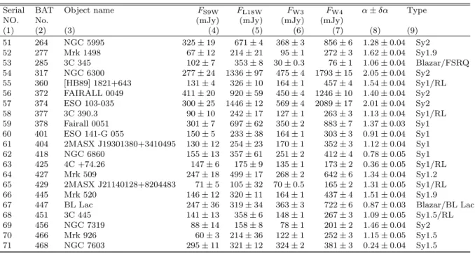
As a result, among 111/129 AGN of theSwift/BAT-AKARI(9/18µm bands) sample, 75 and 109 AGN are detected in W3 (68%) and W4 (84%) bands, respectively. Those not detected in WISEare mostly rejected with the criterion of ”Reduced chi-square”. In what follows, we use only the sources detected in all 4 bands (AKARI/IRC 9 and 18 µm bands and WISEW3 and W4 bands). This leaves a total of 71 sources. As explained in Section 3.2, the 4-band data are essential to correct band difference betweenAKARIandWISE. We summarize parameters of the selected sources (name, IR fluxes, AGN type) inTable 1. Additionally, we list a number of sources for each AGN type in Table 2.
TABLE 1
List of AGN for the current studies and their mid-IR fluxes in theAKARIandWISEcatalog
Serial BAT Object name FS9W FL18W FW3 FW4 α±δα Type
NO. No. (mJy) (mJy) (mJy) (mJy)
(1) (2) (3) (4) (5) (6) (7) (8) (9)
1 1 Mrk 335 128±3 223±46 163±1 310±3 0.98±0.04 Sy1.2
2 21 NGC 526A 141±14 292±26 140±1 308±3 1.21±0.04 Sy1.5
3 22 Fairall 9 229±20 440±24 262±2 468±4 0.90±0.04 Sy1
4 34 NGC 931 349±12 763±48 427±3 977±9 1.25±0.04 Sy1.5
5 35 IC 1816 55±32 265±20 114±1 369±4 1.81±0.05 Sy1.8
6 37 NGC 985 165±14 368±38 176±1 491±5 1.57±0.04 Sy1
7 41 NGC 1052 146±34 377±17 157±1 445±5 1.61±0.05 Sy2/RL
8 43 [HB89] 0241+622 300±14 635±34 365±3 715±6 1.03±0.04 Sy1/RL
9 50 NGC 1194 169±7 415±56 217±1 524±5 1.35±0.04 Sy1
10 54 NGC 1275 442±26 1988±21 751±5 2900±20 2.08±0.03 Sy2/RL
11 72 IRAS 04124-0803 168±12 423±39 213±1 483±5 1.26±0.04 Sy1
12 77 3C 120 203±20 497±68 232±2 590±5 1.43±0.04 Sy1/RL
13 83 CGCG 420-015 173±7 471±22 253±2 566±5 1.25±0.04 Sy2
14 84 ESO 033-G 002 163±7 387±15 188±1 408±4 1.19±0.04 Sy2
15 85 LEDA 097068 218±13 581±27 277±2 788±7 1.61±0.04 Sy1
16 89 Ark 120 252±18 253±33 227±2 339±4 0.61±0.04 Sy1
17 90 ESO 362-18 166±31 366±36 171±1 478±5 1.58±0.04 Sy1.5
18 93 PKS 0521-36 97±0.1 216±20 115±1 245±2 0.94±0.02 Blazar/BL Lac
19 109 NGC 2110 300±19 566±30 371±3 800±6 1.18±0.04 Sy2
20 112 2MASX J05580206-3820043 348±15 536±17 374±3 575±5 0.66±0.04 Sy1
21 125 Mrk 79 276±6 611±38 297±2 737±8 1.29±0.04 Sy1.2
22 133 Phoenix Galaxy 274±19 1310±6 446±3 1772±15 2.20±0.04 Sy2
23 138 FAIRALL 1146 157±14 441±30 196±1 535±5 1.54±0.04 Sy1.5
24 146 Mrk 704 256±30 469±20 284±2 510±6 0.91±0.05 Sy1.5
25 149 MCG +04-22-042 78±15 178±47 104±1 210±2 1.08±0.05 Sy1.2
26 152 Mrk 705 99±21 214±44 109±1 254±3 1.31±0.05 Sy1.2
27 154 MCG -05-23-016 384±14 1391±21 633±4 1843±9 1.65±0.03 Sy2
28 164 NGC 3227 444±71 1128±44 513±4 1516±13 1.67±0.04 Sy1.5
29 165 NGC 3281 415±9 1509±29 670±5 2138±15 1.78±0.03 Sy2/CT
30 167 LEDA 093974 96±23 256±68 88±1 242±2 1.56±0.04 Sy2
31 171 NGC 3516 262±20 651±16 313±2 778±7 1.41±0.04 Sy1.5
32 179 NGC 3783 502±10 1530±41 670±5 2038±11 1.66±0.03 Sy1
33 185 NGC 3998 98±22 133±20 93±1 151±2 0.75±0.05 LINERa
34 187 LEDA 38038 166±8 614±41 260±1 803±4 1.74±0.03 Sy2
35 188 NGC 4051 346±30 885±42 472±4 1153±10 1.38±0.04 Sy1.5 36 196 Mrk 766 220±13 859±20 317±2 1177±11 2.02±0.04 Sy1.5
37 204 3C 273 276±3 454±7 277±2 556±6 1.92±0.06 Blazar/FSRQ 38 206 NGC 4507 510±4 1163±31 550±4 1476±10 1.22±0.02 Sy2
39 222 ESO 323-077 472±3 902±17 523±4 1130±8 0.96±0.02 Sy1.2 40 225 MCG -03-34-064 453±11 1873±45 761±5 2297±16 1.72±0.03 Sy1.8
41 228 MCG -06-30-015 280±32 591±11 334±3 749±7 1.24±0.04 Sy1.2 42 230 4U 1344-60 207±9 556±28 267±2 684±6 1.44±0.04 Sy1.5
43 231 IC 4329A 769±12 1790±34 998±6 2093±16 1.12±0.03 Sy1.2 44 233 Mrk 279 141±9 387±28 143±1 378±3 1.49±0.04 Sy1.5
45 237 NGC 5548 157±5 409±40 189±1 520±4 1.53±0.04 Sy1.5 46 239 SBS 1419+480 46±6 189±13 84±1 238±2 1.60±0.04 Sy1.5
47 241 Mrk 817 188±10 669±27 274±2 940±8 1.89±0.04 Sy1.5 48 246 WKK 4438 94±15 266±12 115±1 325±3 1.60±0.04 Sy1
49 247 IC 4518A 243±27 677±22 240±2 963±8 2.14±0.04 Sy2 50 248 Mrk 841 126±13 372±25 161±1 445±4 1.57±0.04 Sy1
± ± ± ± ±
51 264 NGC 5995 325±19 671±4 368±3 856±6 1.28±0.04 Sy2
52 277 Mrk 1498 67±12 214±21 95±1 272±3 1.62±0.04 Sy1.9 53 285 3C 345 102±7 353±8 30±0.3 76±1 1.06±0.04 Blazar/FSRQ
54 317 NGC 6300 277±24 1336±97 475±4 1793±15 2.05±0.04 Sy2 55 360 [HB89] 1821+643 131±4 326±10 164±1 457±4 1.54±0.04 Sy1/RL
56 372 FAIRALL 0049 411±20 920±59 450±4 1246±10 1.40±0.04 Sy2 57 374 ESO 103-035 300±25 1446±12 569±4 2089±17 2.01±0.04 Sy2
58 377 3C 390.3 90±10 242±17 127±1 263±3 1.13±0.04 Sy1/RL 59 378 Fairall 0051 301±7 697±62 350±2 883±7 1.37±0.03 Sy1
60 401 ESO 141-G 055 150±5 233±38 164±1 303±3 0.91±0.04 Sy1
Note. — Col. 1: serial number. Col. 2: Object number in the 22-monthSwift/BAT hard X-ray survey catalog (Tueller et al. 2010).
Col. 3: Object name. Col. 4 and 5: The flux and error in S9W (9µm) and L18W (18µm) taken from theAKARI/PSC in units of mJy.
Col. 6 and 7: The flux and error in W3 (12µm) and W4 (22µm) taken from theWISEAll-sky Source Catalog in units of mJy. Col. 8:
The slope and error of the SED of each source Col. 9: Optical AGN type taken from Tueller et al. (2010) or from other literature as listed below:
References. — a
V´eron-Cetty & V´eron (2010);
TABLE 1
Continued.
Serial BAT Object name FS9W FL18W FW3 FW4 α±δα Type
NO. No. (mJy) (mJy) (mJy) (mJy)
(1) (2) (3) (4) (5) (6) (7) (8) (9)
1 352±3 1.12±0.04 Sy1
2 412±4 0.78±0.05 Sy1
1 173±2 0.36±0.05 Sy1/RL
2 642±6 1.34±0.04 Sy1.2
5 165±2 1.31±0.05 Sy1/RL
1 437±4 1.51±0.04 Sy1.9
3 722±6 0.87±0.03 Blazar/BL Lac
1 267±3 1.09±0.05 Sy1.5/RL
1 201±2 1.46±0.04 Sy2
1 252±3 1.15±0.05 Sy1.5
2 381±3 0.24±0.04 Sy1.5
61 404 2MASX J19301380+3410495 130±12 254±23 170±1
62 418 NGC 6860 155±13 357±61 251±2
63 425 4C +74.26 147±6 175±9 135±1
64 427 Mrk 509 247±18 499±17 268±2
65 429 2MASX J21140128+8204483 71±5 105±32 70±0.5
66 445 Mrk 520 146±12 320±11 164±1
67 447 BL Lac 247±36 319±34 363±3
68 451 3C 445 141±13 358±6 148±1
69 456 NGC 7319 88±14 158±8 78±1
70 466 Mrk 926 60±3 214±36 122±1
71 468 NGC 7603 295±11 321±12 324±2
TABLE 2
Number of cross-identified AGN for each type
Source type total
Sy1 Sy2 LINER BL RL1 RL2 CT
(1) (2) (3) (4) (5) (6) (7) (8)
38 18 1 4 7 2 1 71
Note. — Col. 1–7: Numbers of detected sources in 4-bands ofAKARIand WISEfor each AGN type. Col. 1: Seyfert 1 including
Seyfert 1.2 and 1.5. Col. 2: Seyfert 2 including Seyfert 1.8 and 1.9. Col. 3: LINERs. Col. 4: Blazars. Col. 5: type 1 radio-loud AGN. Col. 6: type 2 radio-loud AGN. Col. 7: Compton-thick AGN. Col. 8: Total numbers of cross-identified sources, i.e., sum of columns 1 through 7.
3. ANALYSIS AND RESULTS
3.1. Relative flux variations
We use relative flux ratios between AKARI and WISE as a basic quantity to describe the time variation of the sources. However, we do not use them directly, but only after applying various corrections as detailed later. The relative flux ratio of thei-th source,Ri
r, is defined as:
Rir=
FWi −F i A Fi
A
, (2)
where FWi andF i
A are fluxes ofi-th source in WISE andAKARI catalogs, respectively. Because of the proximity of the central wavelengths, we compare fluxes ofWISE 12µm (W3) withAKARI 9µm (S9W), andWISE22µm (W4) with AKARI 18 µm (L18W), respectively. Thus we obtain two sets of relative flux rations; one in S9W-W3 band and the other in L18W-W4 band. As the central wave lengths of the data, we use the isophotal wavelengths defined as 8.61, 11.56, 18.39, and 22.09 µm for S9W, W3, L18W, and W4, respectively (Ishihara et al. 2010; Wright et al. 2010). Because the observation bands of AKARI and WISE are slightly different, the difference must be corrected; the correction method will be explained in the next subsection§3.2.
3. ANALYSIS AND RESULTS
3.1. Relative flux variations
TABLE 1
§
3.2. Correction of the band differences
We calculate a correction factor due to the band difference for each source using the SED. We assume that the SED has a power-law form, which is a good approximation for AGN except for local emission/absorption structures. We use AKARIand WISEdata themselves to determine the power-law slope of the SED. Of course, because the source may be time variable, AKARI andWISE data may show systematic offset. However, the power-law slope of SED is considered to be rather insensitive to the time variation. Because of the proximity of the correspondingAKARI and
WISE bands, the slope is basically determined to connect the weighted average of W3 and S9W fluxes and that of W4 and L18W fluxes. In reality, theWISE data have much better statistics than theAKARIdata. Thus the slope is mostly determined by the WISEdata. We use the isophotal wavelengths described in the previous subsection as the center of the wave bands, and ignored their errors.
Once the slope is determined, we can calculate the correction factor,Ri
c, to the relative flux ratio as follows,
Ric= (
λW
λA )α
i
−1, (3)
whereλW andλAare the isophotal wavelengths ofWISEandAKARI, respectively. αi is the slope of the SED ofi-th source. In addition, the error ofRi
c,δR i
c, is calculated as,
δRic= ( λW λA )α i log ( λW λA )
×δαi, (4)
whereδαi
is the error ofαi
. Average values ofRi
c were 0.49 and 0.29 in S9W-W3 and L18W-W4, respectively, for the whole samples, and those of errors were 7×10⁻³
and 4×10⁻³
, respectively. We calculatedRi
r−R i
c for each source and evaluated their distribution. However, the center of the distribution in S9W-W3 bands calculated for the whole sample was −0.25, significantly offset from zero. Similar tendency was also seen in the L18W-W4 band with smaller magnitude (−0.04). Several reasons may be conceivable for the offsets: for example, shifts of the center of the wave bands from the isophotal values due to the different slope from Vega, and the local structures of the emission/absorption lines. We represent the offsets as r, and will subtract it from the relative flux ratios in the subsequent analysis.
3.3. Variability criteria
Using the relative flux ratios, we search the catalogs for variable sources. For this purpose, we normalize the ratios with the errors, because the normalized ratios are directly related to the significance of variations. Thus, we introduce variability criteriaSfollowing Enya et al. (2002c) as follows:
Si= R i r−R
i c−r √
δRi r
2 +δRi
c
2. (5)
Here, Ri
ris the relative flux ratio defined in Equation (2),R i
c andδR i
c are the correction to the relative flux ratio due to the wave band difference and its error, respectively,ris an average ofRi
r−R i
c defined for the total samples or each subtype depending on the samples under consideration. δRi
ris an error of R i
r defined as:
(δRi r
Ri r
)2 =
(δFi W Fi
W )2
+ (δFi
A Fi
A )2
+ϵ2 (6)
where FWi andFAi areWISEand AKARIfluxes, respectively, andδFWi andδFAi are their respective errors. We also introduced a constant factor,ϵ, to incorporate the cross-calibration error betweenAKARIandWISE. Cross-calibration analysis was done to evaluateϵ, which is described in Appendix. ϵis independent of types of the source, and is 1.5% and 4.1% for the S9W-W3 and L18W-W4, respectively. We note that the errors δRi
r and δR i
c are in reality not independent. This is because δRci is determined by δαi, which originate from the errors of FWi and FAi. Thus the denominator of Equation (5) may be slightly overestimated. However, we adopted the definition of Equation (5) as this is conservative way to evaluate the significance of variability.
We show frequency distribution of S in a bar chart in Figure 1 for the S9W-W3 and L18W-W4 bands. It is clear that most of AGN have S concentrated aroundS= 0 with a few exceptions. These exceptional sources are strongly time variable ones. We list largely deviated sources with > 8σ confidence limit, i.e., |S| >8, in Table 3 (2 blazars and 1 RL1). The criterion of 8σ is selected rather arbitrarily, but is large enough to exclude any marginal sources. These are the best candidates of variable sources. Only 1 source, which is a blazar, shows significant variability in both bands.
After excluding significantly variable sources in Table 3, we calculated the standard deviation and error ofS for the remaining samples. The standard deviation was 2.36±0.20 and 1.17±0.10 in the S9W-W3 and L18W-W4, respectively. Here, the errors represent 1σ confidence limit. It is immediately noticed that the standard deviation is significantly larger than unity for the S9W-W3 band. This means that the sample distribution in the S9W-W3 is much larger than
3.2. Correction of the band differences
that expected from the pure statistical variations of the sources. On the other hand, the sample distribution in the L18W-W4 may be consistent to the pure statistical one. In order to evaluate the presence of extra scattering in the data, it is crucial to estimate the confidence interval of the standard deviations accurately. Calculation of the error of standard deviations assumes normal distribution of the data, which is not necessarily true in this case. Thus, we applied the bootstrap method to estimate the reliable confidence interval of the standard deviations. In the bootstrap method, no a priori assumption is made for the parent distribution of the data. The data themselves, Sin this case, are assumed to compose the parent distribution, and samples are selected randomly allowing redundancy. This trial is repeated many times (2000 times in this case) to determine the confidence interval. The bootstrap method is applied for both S9W-W3 and L18W-W4 bands. We summarize all the results in Table 4. We could not calculate averages and standard deviations for CT AGN and LINER in both bands because the available sample is only one. Similarly, the results may not be reliable for RL2 and BL because of the small number of samples. The table also includes the errors of the standard deviations calculated assuming the normal distribution of the samples, i.e., standard deviation divided by √
2(N−1), where N is the number of samples. It is clear from the table that the standard deviation in
the S9W-W3 band is significantly larger than unity for the whole category and for Seyfert 1s and 2s. This means that Seyferts as a whole may be more or less variable in the S9W-W3 band, although the time variations are difficult to detect individually. We evaluate the magnitude of time variations in the next subsection.
−30 −20 −10 0 10
0
5
10
15
Frequency
Variability criterion, S (S9W−W3)
−60 −40 −20 0
0
10
20
Frequency
Variability criterion, S (L18W−W4)
Fig. 1.—Distribution of the variability criteria, Sdefined in Equation 5. The abscissa showsS of each source, and the ordinate the
number of sources. The left and right panels are histograms in the S9W-W3 and L18W-W4 bands, respectively. Total number of sources are both 71. In both histograms, the bin size is set to ∆S= 1.
TABLE3
Sources variable at>8 sigma significance level
Object name FS9W FL18W FW12 FW22 S Type
(mJy) (mJy) (mJy) (mJy) S9W-W3 / L18W-W4
(1) (2) (3) (4) (5) (6) (7)
3C 345 102±7 353±8 30.1±0.3 76±1 –28.8 / -66.0 Blazar
3C 273 276±3 454±7 277±2 556±6 -15.6 / -2.6 Blazar
3C 445 141±13 358±6 148±1 267±3 -0.9 / -11.3 type1 RL
Note. — Col. 1: Object name. Col. 2–3: Flux and error in the S9W and L18W bands taken from theAKARIcatalog in units of mJy.
Col. 4–5: Flux and error in the W3 and W4 bands taken fromWISEall-sky source catalog in units of mJy, which are converted from that in units of magnitude by Equation 1. Col. 6: Variability criteria in the S9W-W3 and L18W-W4 bands estimated by Equation 5. Col. 7: Optical AGN type taken from Tueller et al. (2010); here RL means radio-loud AGN.
TABLE 3 FIG. 1.
variation of the sample as follows:
σint
D
2
= 1
N−1 n ∑
i=1
{(Di−D¯)2
−(δsD
i
)2
}. (10)
In this definition ofσint
D , contribution from the statistical variation is subtracted. The results are summarized in Table 5,
in which the confidence intervals ofσint
D are calculated with two methods, one assuming the normal distribution of the
samples and the other using the boot strap method. We found that Seyfert 1 in the S9W-W3 band show significant variability of 13% (6–18%) in 95% confidence limit. Seyfert 2 and RL1 AGN show a hint of variability, but the significance is low.
3.4. Fractional variability in mid-IR band
In order to quantify the time variations of the sample as a whole, we introduce the fractional variation defined as the flux variation normalized by the weighted-mean average flux. They are defined as:
Di=F
i
W −(1 +R i c+r)F
i A
Fi (7)
Fi=δF i A
2
FWi +δFWi 2(1 +Ric+r)FAi
δFi A
2
+δFi W
2 (8)
Here, Di is the fractional variation, in which the weighted-mean flux ¯Fi is used to normalize it. In this analysis, we
excluded significantly variable sources in Table 3. We show frequency distribution ofDi
in a bar chart in Figure 2 for the whole samples. The width of the distribution indicates the relative variability of the samples, but caution should be paid to the contribution of the statistical errors. The width results from both the statistical variations and the intrinsic time variations. The former is defined by the statistical errors of the data. The statistical variations of Di, which is denoted as δsDi hereafter, is estimated as
follows:
(δsDi) 2
= {(δFi
W
Fi )2
+
(1 +Ri c+r
Fi δF
i A
)2}
(9)
Here we ignore errors of Ri
c and Fi, because they originate from the errors of F i
W and F i
A and do not compose of
independent errors. Using this equation, we define, σint
D , the standard deviation corresponding to the intrinsic time
TABLE 4
Averages and standard deviations of the variability criteriaSand their confidence intervals
Type N S
average standard deviation confidence interval (95%) normal dist. boot strap
(1) (2) (3) (4) (5) (6)
S9W-W3 band
All 69 0.00±0.19 2.36 1.97–2.75 1.92–2.75 Sy1 38 −0.11±0.12 2.33 1.80–2.86 1.63–2.89 Sy2 18 −0.15±0.31 2.69 1.79–3.59 1.74–3.37 RL1 7 −0.10±0.10 1.77 0.77–2.77 0.93–2.17
RL2 2 0.47±0.20 1.69 – –
CT 1 · · · ·
LI 1 · · · ·
BL 2 7.97±0.16 7.30±5.16 – – L18W-W4 band
All 69 0.01±0.14 1.17 0.97–1.37 0.88–1.43 Sy1 38 −0.11±0.14 1.00 0.76–1.24 0.66–1.32 Sy2 18 0.10±0.11 1.14 0.77–1.51 0.74–1.41 RL1 6 0.25±0.22 0.98 0.37–1.59 0.24–1.29
RL2 2 0.09±0.07 1.51 – –
CT 1 · · · ·
LI 1 · · · ·
BL 3 0.54±0.17 3.47±1.74 0.06–6.88 <3.96
Note. — Col. 1: Object type. Col. 2: Number of sources in each subtype, from which significantly variable sources listed in Table 3 are excluded. Col. 3: Average and error of variability criteria,S. Col. 4: standard deviation of variability criteria,S. Col. 5: Confidence
interval of the standard deviation in 95% confidence limit calculated assuming the normal distribution of the samples. Col.6: Same as column 5 but calculated using the boot strap method.
3.4. Fractional variability in mid-IR band
−50 0 50
0
5
10
15
Frequency
Relative flux variations, D (S9W−W3) [%]
−50 0 50
0
10
20
Frequency
Relative flux variations, D (L18W−W4) [%]
Fig. 2.—Frequency distribution of the relative flux variations for the total sample of AGN in the S9W-W3 band (left panel) and L18W-W4 band (right panel). The abscissa shows relative flux variations,Di
, in units of %. The ordinate shows the number of sources.
TABLE5
Standard deviations of the fractional variability due to the intrinsic time variations,σint
D, and their confidence intervals
Type N variability fraction
standard deviation confidence interval (95%)
% normal dist. boot strap
(1) (2) (3) (4) (5)
S9W-W3 bands
All 69 14.4 11.3–17.5 7.9–19.5
Sy1 38 13.2 9.5–16.9 6.2–18.0
Sy2 18 19.5 10.9–28.1 <28.4
RL1 7 11.5 3.2–19.8 <16.5
RL2 2 <14.4 – –
CT 1 · · · ·
LI 1 · · · ·
BL 2 <3.1 — —
L18W-W4 bands
All 69 5.2 3.2–7.2 <19.5
Sy1 38 <1.0 <1.8 <6.1
Sy2 18 4.2 0.5–7.9 <12.3
RL1 6 <3.8 <2.1 <7.0
RL2 2 6.7 <18.5 –
CT 1 · · · ·
LI 1 · · · ·
BL 3 32.7 <65.6 <35.6
Note. — Col. 1: Object type. Col. 2: Number of sources in each subsample, from which the variable sources in Table 3 are excluded.
Col. 3: standard deviation of fractional variability. Col. 4: Confidence interval of the standard deviation in 95% confidence limit calculated assuming the normal distribution of the samples. Col.5: Same as column 4 but calculated using the boot strap method.
4. DISCUSSION
We studied time variability of AGN in mid-IR bands combining the all-sky survey catalogs ofAKARI and WISE.
We found 3 significantly variable sources (2 blazars and 1 RL1) in addition to the variability of Sy1 as a whole reaching 6–18% in a relative amplitude in the S9W-W3 band. We discuss possible systematics in the calculation first, then the implication of the results for the individual sources and for Sy1 as a whole.
4.1. Other systematics
Although we have accounted for many systematic effects in comparing theAKARI andWISE catalogs, there may
be some other small effects remaining, e.g., differences of the PSFs, or read out noise. The aperture radius ofAKARI
is 7′′.5 in S9W and L18W. On the other hand, we used results of the profile-fit photometry by WISE whose FWHM
is 6′′.5 and 12′′.0 in W3 and W4, respectively. In order to evaluate systematics due to the difference of the PSFs
betweenAKARIandWISE(i.e., aperture and profile-fit photometry), we calculated flux ratios between the aperture
′′ ′′
4. DISCUSSION
4.1. Other systematics
FIG. 2.
betweenAKARIandWISE(i.e., aperture and profile-fit photometry), we calculated flux ratios between the aperture
and the profile-fitt photometry of WISE. We used aperture magnitudes measured for 8′′.25 and 11′′.0 in radius in W3
and W4, respectively, which are the closest radii to those of AKARI. The average flux ratios of profile-fit-to-aperture
photometry were 1.00 and 1.44 in W3 and W4, respectively. Note that offsets of the flux ratios from 1.0 is not
important because they were subtracted asr in the course of the calculation. The standard deviation of the average
flux ratio was 0.002 and 0.034 in W3 and W4, respectively. The small value of the standard deviation means that the effect of the difference of photometry is negligible than variability.
4.2. Variable sources in mid-IR band 4.2.1. Blazars
Among the 3 variable sources, two are 3C 345 and 3C 273, famous blazars/FSRQs. 3C 345 was highly variable in
both S9W-W3 and L18W-W4 bands, and its fractional variation reached∼300% and 400% in the respective band.
On the other hand, 3C 273 was variable only in S9W-W3 band with a fractional variation of ∼50%.
3C 345 is observationally known to be highly variable in all wave bands including mid-IR. Although observations were rather sparse in mid-IR, time variations of an order of magnitude was clearly detected. Time variations of 60–70%
in a few years were observed in the monitoring at Palomar Observatory at 1.2–10.2µm (Bregman et al. 1986). They
generally had corresponding events in the optical band. Similar amplitude of variations (∼50% in 12–25µm) in a few
months were observed by pointed IRASobservations (Edelson & Malkan 1987). The monitoring campaign from radio
through optical bands in 2005-2006 showed the evolution of SEDs with mid-IR variations reaching ∼100% in a few
years (Bach et al. 2007). Large time variations we detected in the mid-IR bands, a factor of ∼3–4 in 4 years, may be
regarded as one of the typical behaviors of 3C 345.
3C 273 is a famous, bright, and nearby blazar and is well studied at all wavelengths (Courvoisier 1998). Monitoring
observations over two decades at 10.6µm, revealed time variations of∼1 mag in a few years (Neugebauer & Matthews
1999). The monitoring campaign from radio through optical bands in 2005-2006 showed the evolution of SEDs which
may correspond to mid-IR variations of∼50% in a few years (Bach et al. 2007). Characteristics of blazar in 3C 273
may be more clearly recognized at near-IR than at optical wavelengths. Monitoring observations for 4 years in the near-IR and radio bands detected several flares, in which the near-IR fluxes increased by a factor of a few (Robson et
al. 1993). McHardy et al. (1999) showed that the X-ray (3-20 keV) and near-IR (K band, 2.2µm) variations of 3C 273
were highly correlated. The strong correlation supports the synchrotron self-Compton model, where the seed photons of near-IR band are synchrotron photons from the jets. Compared to these past observations, significant variations we detected from 3C 273 in the S9W-W3 band (∼50% in 4 years) may be typical of this source.
Both blazars are monitored frequently inR-band with two nearly identical photometers-polarimeters of AZT-8 (the
Crimean Observatory, Ukraine) and LX-200 (St. Petersburg University, Russia) since 2005 or 2006. The light curves
of 3C 3452
and 3C 2733
both show flaring events superposed on the gradual variations. Because the light curves cover theAKARIandWISEsurvey periods, we can roughly infer the R-band variations between these two surveys: ∼1 mag
decrease for 3C 345 and∼0.2 mag decrease for 3C 273. Although direct comparison is difficult due to the wavelength
difference, the decreasing trend in the R-band is consistent to our mid-IR results (S<0).
4.2.2. Radio-loud AGN
3C 445 is a nearby (z= 0.056) FR II radio galaxy (Hewitt & Burbidge 1991; Kronberg et al. 1986). We detected a flux decrease of ∼50% in L18W-W4 band whereas the decrease was insignificant at ∼9% in S9W-W3 band. Similar variation in mid-IR emission from 3C 445 is not reported so far.
Origin of the mid-IR emission from radio-loud AGN is not well understood yet. From the comparison of SEDs between BLRGs and a blazar (3C 273), Grandi & Palumbo (2007) suggested that although the jet contribution in X-ray band does not exceed 45%, the SEDs of powerful BLRGs likely hide a jet with a spectral shape very similar to that of 3C 273, and the IR bump of radio galaxies recalls the synchrotron peak of blazars. On the other hand, from the statistical analysis of 19 3CRR radio-loud galaxies including 3C 445 in mid- to far-IR observations, Dicken et al. (2010) concluded that the dominant heating mechanism for mid-IR emitting dust is AGN illumination based on the correlation between mid-IR luminosities and the AGN power indicator [OIII].
If we invoke only the AGN illumination, the large fractional variation (∼50%) detected from 3C 445 may be difficult to explain. According to the clumpy torus variability model of type 1 AGN (H¨onig & Kishimoto 2011), variation in L18W-W4 bands is predicted to be much smaller than that detected from 3C 445, even if a very strong AGN flare with 50% total luminosity were to be occur. The large variability observed from 3C 445 may instead be interpreted as the contribution of the non-thermal emission from the jet.
4.3. Fractional variability for each type of AGN
Through the analysis of fractional variability in Section 3.4, we found that Sy1 show variability∼13% (6-18%) in S9W-W3 bands at the 95% confidence limit. Heretofore, few data exist on 10 µm variability on long timescales for Seyferts. In a two decade long multiwavelength monitoring campaign, Neugebauer & Matthews (1999) found a mean variability of ∼10% at 10µm from 25 radio-quiet quasars. Our result indicates for the first time that Sy1 may have intrinsically similar variability as quasars in the mid-IR band.
We could not detect significant variations from other subsamples mostly due to the limited statistics. However, this 4.2. Variable sources in mid-IR band
4.2.1. Blazars
4.2.2. Radio-loud AGN
4.3 Fractional variability for each type of AGN
does not exclude the presence of similar variability as Sy1 for other types of AGN. This is true especially for Sy2, whose upper limit of fractional variations in S9W-W3 band was 28%. Thus our results allow presence of similar time variations in Sy1 and Sy2.
4.4. Variability time scale of torus emission
Because the IR emission from Sy is considered to originate from the dusty torus illuminated by AGN, we first try to interpret the variability we detected from Sy1 as that of the torus emission. The thermal equilibrium relation of graphite grains may be used to give the dust location as a function of its temperature as,
r=1.3 3
( L
UV
1046erg s−1
)1/2( T 1500 K
)−2.8
pc, (11)
whereris the distance from the central region,LUVis the UV luminosity,T is the grain temperature (Barvainis 1987). We included in this equation a factor of ∼1/3 (Kishimoto et al. 2007; Nenkova et al. 2008; Kawaguchi & Mori 2010) as indicated by the time lag measurements of four nearby Sy1 galaxies by Suganuma et al. (2006).
If we assume a central X-ray luminosity of 1044 erg s−1
, which is a median value of our sample of AGN, the luminosity in UV band may be estimated as ∼(2–3)×1045 erg s−1 (Elvis et al. 1994; Vasudevan & Fabian 2007). Using this UV
luminosity, dust grains at 300 K, whose emission peaks at 9 µm, are estimated to lie 10 pc (∼30 light-year) from the central region. If we interpret this distance naively, it seems to be too large compared to the rapid time variations we detected (∼13% in 4-years). However, a detailed model is required to make quantitative evaluation whether the distance is indeed incompatible with our result of time variations. Such detailed modeling is out of the scope of the present paper, but we show an example of the model from the literature in the next subsection and discuss a possible constraint on the dust distribution.
4.5. Dust distribution in the torus
According to the variability model of type 1 AGN (H¨onig & Kishimoto 2010, 2011), time variation in the mid-IR band as a response to the variation of the incident radiation on the torus is largely dependent on dust distribution in the torus. H¨onig & Kishimoto (2011) defined dust distribution in the torus with the surface filling factor which has a radial dependence of rα. When dust distribution is flat (α > −0.5), their simulation shows no clear peak in the
mid-IR band (8.5µm in their simulation) as a response to the step function change of the incident AGN radiation. On the other hand, if dust distribution is narrow (α <−1.5), i.e., its distribution is limited in terms of the distance from
the AGN, the mid-IR emission shows delayed peak in the light curve. The time scale of mid-IR variations near the peak can be shorter than the light crossing time of the torus. In this case, the mid-IR emission is dominated by the Rayleigh-Jeans tail of the hot dust emission located in the inner torus, not by the peak blackbody emission of cooler dust. Although this is rather simplified view of time variations, if the mid-IR variability can be explained by the torus emission only, those detected in Sy1 (∼13% in 4 years) prefer rather narrow distribution of dust in the torus. The mid-IR variability will become a useful tool to constrain dust distribution in AGN tori.
4.6. Other origins of variability
The variability we detected from Sy1 may have different origin than the torus. Here we consider the possibility of jet contribution. Most of Seyfert 1 show some degree of radio-loudness, which is inferred from the nuclear radio-to-optical luminosity ratios (Ho & Peng 2001). Also, elongated jet-like features were discovered from 14 Seyferts by the Very Large Array (VLA) surveys (Ho & Ulvestad 2001). Recently ejected jet may contribute to mid-IR variability. If this is the case, the jet activity should be observed with recent and future all-sky surveys in the radio band such as the LOw Frequency ARray (LOFAR) and the square Kilometer Array (SKA).
5. CONCLUSIONS
We studied mid-IR variability of AGN systematically in order to constrain the geometry of the dusty torus. Com-bining two sets of all-sky survey data fromAKARIandWISE, we calculated time variations of each source excluding the systematic effects as much as possible. As a result, we found 3 sources, 2 blazars and 1 RL1, significantly variable in the mid-IR band. We also estimated average variability for each type of AGN excluding the three variable sources. We found that Sy1 show significant variability of∼13% (6–18% in the 95% confidence interval) in the S9W-W3 band. Comparing the detected variation (13% in 4 years) with the model calculation for the type 1 AGN, we conjectured that, if the variation results from the torus, dust distribution in the torus should be narrow. Alternatively, it is also possible that the variation originates from the jets in Sy1, whose presence is suggested from the radio observations.
This research is based on observations withAKARI, a JAXA project with the participation of ESA. In addition, this pub-lication makes use of data products from the Wide-field Infrared Survey Explorer, which is a joint project of the University of California, Los Angeles, and the Jet Propulsion Laboratory/California Institute of Technology, funded by the National Aeronautics and Space Administration.
4.4 Variability time scale of torus emission
4.5 Dust distribution in the torus
4.6 Other origins of variability
REFERENCES Bach, U., Raiteri, C. M., Villata, M., et al. 2007, A&A, 464, 175
Barvainis, R. 1987, ApJ, 320, 537
Bregman, J. N., Glassgold, A. E., Huggins, P. J., et al. 1986, ApJ, 301, 708
Clavel, J., Wamsteker, W., & Glass, I. S. 1989, ApJ, 337, 236 Courvoisier, T. J.-L. 1998, A&A Rev., 9, 1
Dicken, D., Tadhunter, C., Axon, D., et al. 2010, ApJ, 722, 1333 Edelson, R. A., & Malkan, M. A. 1987, ApJ, 323, 516
Elvis, M., Wilkes, B. J., McDowell, J. C., et al. 1994, ApJS, 95, 1 Enya, K., Yoshii, Y., Kobayashi, Y., et al. 2002, ApJS, 141, 23 Enya, K., Yoshii, Y., Kobayashi, Y., et al. 2002, ApJS, 141, 31 Enya, K., Yoshii, Y., Kobayashi, Y., et al. 2002, ApJS, 141, 45 Gorjian, V., Werner, M. W., Jarrett, T. H., Cole, D. M., &
Ressler, M. E. 2004, ApJ, 605, 156
Grandi, P., & Palumbo, G. G. C. 2007, ApJ, 659, 235 H¨onig, S. F., & Kishimoto, M. 2010, A&A, 523, A27 H¨onig, S. F., & Kishimoto, M. 2011, A&A, 534, A121 Haardt, F., & Maraschi, L. 1993, ApJ, 413, 507 Hewitt, A., & Burbidge, G. 1991, ApJS, 75, 297 Ho, L. C., & Peng, C. Y. 2001, ApJ, 555, 650 Ho, L. C., & Ulvestad, J. S. 2001, ApJS, 133, 77
Hoffman, D. I., Cutri, R. M., Masci, F. J., et al. 2012, AJ, 143, 118
Hunt, L. K., Zhekov, S., Salvati, M., Mannucci, F., & Stanga, R. M. 1994, A&A, 292, 67
Ishihara, D., et al. 2010, A&A, 514, A1
Jarrett, T. H., Cohen, M., Masci, F., et al. 2011, ApJ, 735, 112 Kawaguchi, T., & Mori, M. 2010, ApJ, 724, L183
Kishimoto, M., H¨onig, S. F., Beckert, T., & Weigelt, G. 2007, A&A, 476, 713
Koz�lowski, S., Kochanek, C. S., Stern, D., et al. 2010, ApJ, 716, 530
Kronberg, P. P., Wielebinski, R., & Graham, D. A. 1986, A&A, 169, 63
Matsuta, K., Gandhi, P., Dotani, T., et al. 2012, ApJ, 753, 104 McHardy, I., Lawson, A., Newsam, A., et al. 1999, MNRAS, 310,
571
Murakami, H., Baba, H., Barthel, P., et al. 2007, PASJ, 59, 369 Nenkova, M., Sirocky, M. M., Nikutta, R., Ivezi´c, ˇZ., & Elitzur,
M. 2008, ApJ, 685, 160
Neugebauer, G., Soifer, B. T., Matthews, K., & Elias, J. H. 1989, AJ, 97, 957
Neugebauer, G., & Matthews, K. 1999, AJ, 118, 35
Robson, E. I., Litchfield, S. J., Gear, W. K., et al. 1993, MNRAS, 262, 249
Suganuma, M., Yoshii, Y., Kobayashi, Y., et al. 2006, ApJ, 639, 46
Tueller, J., et al. 2010, ApJS, 186, 378
Ulrich, M.-H., Maraschi, L., & Urry, C. M. 1997, ARA&A, 35, 445 V´eron-Cetty, M.-P., & V´eron, P. 2010, A&A, 518, A10
Vasudevan, R. V., & Fabian, A. C. 2007, MNRAS, 381, 1235 Wright, E. L., Eisenhardt, P. R. M., Mainzer, A. K., et al. 2010,
AJ, 140, 1868
Yamamura, I., Makiuti, S., Ikeda, N., Fukuda, Y., Oyabu, S., Koga, T., & White, G. J. 2010, VizieR Online Data Catalogue, 2298, 0
APPENDIX
RELATIVE CALIBRATION ERRORS BETWEENAKARIANDWISE
When comparing observed fluxes between different satellites, it is important to consider the relative calibration error accurately because the cataloged fluxes usually include various systematic effects. Therefore, we estimate relative calibration error between AKARI and WISE using bright stars commonly detected with these two satellites. We selected A- and F-type stars for this purpose (115/145 and 150/178 sources in S9W-W3/L18-W4) because their spectra in IR bands are rather featureless and are well approximated by a blackbody. As we need to use only bright stars to minimize the statistical errors, we plot the Signal-to-Noise ratio (S/N) of AKARI for A- and F-type stars commonly detected by AKARI and WISE in Figure 3. We select bright stars based on the following criteria on the
AKARI fluxes:
• Flux>800 mJy, and S/N >50 in theAKARI S9W band; this leaves 38/57 sources for A-/F- type,
• Flux>300 mJy, and S/N >10 in theAKARI L18W band; this leaves 40/34 sources for A-/F- type.
Here, S/N is defined as the flux divided by its error.
We calculate relative flux ratioRr defined in Equation 2 for the selected bright stars, and show the distributions
in Figure 4. We then determined the center of the distribution by fitting a Gaussian; the results are summarized in Table 6. The non-zero values of Rr are mostly due to the band difference betweenAKARI and WISE. Thus we
calculate the relative flux ratioR′
r due to the band difference for pure blackbody emission. If we assume temperature
of F0 star (7200 K), R′
r is calculated as -0.428 and -0.301 in S9W-W3 and L18W-W4, respectively. Note that these
values are rather insensitive to the selection of temperature, because the observation bands lie in the Rayleigh-Jeans region. The differencesRr−R′rbetween the observed and calculated values represent the calibration errors, and were
–0.015 and –0.041. Therefore, we estimate the relative calibration error, |(R′
r−Rr)/R′r|betweenAKARI andWISE
as 1.5% and 4.1% in S9W-W3 and L18W-W4, respectively.
100 1000
1
10
100
1000
Signal to Noise Ratio
Flux (9µm band) [mJy] A−type star
F−type star
100 1000
1
10
100
1000
Signal to Noise Ratio
Flux (18µm band) [mJy]
A−type star
F−type star
Fig. 3.—Signal-to-Noise (S/N) ratio, defined as theAKARIflux divided by its error, of A- and F-type stars detected by bothAKARI
andWISEare plotted against theAKARIfluxes. Left panel is for the S9W band and right panel for the L18W band. Black circles indicate
A-type stars and red squares F-type stars. Bright stars with good S/N ratio, located in the upper-right region as indicated by the broken lines, are used for the estimation of the relative calibration error.
TABLE 6
Summary ofRr calculation
Wave band Number of stars Relative flux ratio
AKARI-WISE A/F type Rr R′r R′r−Rr
S9W-W3 38/57 -0.443 -0.428 -0.015
L18W-W4 40/34 -0.342 -0.301 -0.041
APPENDIX
FIG. 3.
13
−0.5 −0.45 −0.4 −0.35
0
10
20
30
Number of stars
Rr (S9W−W3)
−1 −0.5 0 0.5 1
0
10
20
Number of stars
Rr (L18W−W4)
Fig. 4.—Distribution of the relative flux ratioRr betweenAKARI andWISEfor the sum of A- and F-type stars. Left panel shows
the distribution for S9W-W3 band, and right panel for L18W-W4 band. Broken line shows the best-fit Gaussian model, which is used to determine the center of the distribution.
Edited and Published by: Japan Aerospace Exploration Agency
7-44-1 Jindaiji-higashimachi, Chofu-shi, Tokyo 182-8522 Japan URL: http://www.jaxa.jp/
Date of Issue: February 13, 2017 Produced by: Matsueda Printing Inc.