PAPER
Special Section on Parallel and Distributed Computing and NetworkingAn FPGA-Based Change-Point Detection for 10Gbps Packet Stream
Takuma IWATA†a), Kohei NAKAMURA†, Yuta TOKUSASHI†,Nonmembers, andHiroki MATSUTANI†,Member
SUMMARY In statistical analysis and data mining, change-point de- tection that identifies the change-points which are times when the prob- ability distribution of time series changes has been used for various pur- poses, such as anomaly detections on network traffic and transaction data.
However, computation cost of a conventional AR (Auto-Regression) model based approach is too high and infeasible for online. In this paper, an AR model based online change-point detection algorithm, called Change- Finder, is implemented on an FPGA (Field Programmable Gate Array) based NIC (Network Interface Card). The proposed system computes the change-point score from time series data received from 10GbE (10Gbit Ethernet). More specifically, it computes the change-point score at the 10GbE NIC in advance of host applications. It can find change-points on single or multiple streams using a context memory. This paper aims to reduce the host workload and improve change-point detection perfor- mance by offloading ChangeFinder algorithm from host to the NIC. As evaluations, change-point detection in the FPGA NIC is compared with a baseline software implementation and those enhanced by two network opti- mization techniques using DPDK and Netfilter in terms of throughput. The result demonstrates 16.8x improvement in change-point detection through- put compared to the baseline software implementation. It is corresponding to the 10GbE line rate. Performance and area overheads when supporting multiple streams are also evaluated.
key words: Change-point detection, FPGA NIC, 10GbE
1. Introduction
Due to advances in information and communication technol- ogy, datasets exchanged over networks are growing rapidly in the size and the number. As the data sets grow, high- bandwidth becomes more important for data analysis and pattern recognition. Change-point detection is a method to identify the change-points which are times when the prob- ability distribution of time series changes. Popular applica- tions of the change-point detection are related to a security field[1], such as detecting a sudden increase in traffic vol- ume by computer virus and worm. It is also used in other application fields, such as transaction data, resource man- agement, and trend analysis[2].
In a conventional change-point detection algorithm[3], time series data are divided into two sets at time t. Then AR (Auto-Regression) model is built for each set in addi- tion to whole data. Timet is detected as a change-point if a measured error in the whole model is larger than the sum
Manuscript received January 7, 2019.
Manuscript revised May 30, 2019.
Manuscript publicized July 23, 2019.
†The authors are with Graduate School of Science and Tech- nology, Keio University, Yokohama-shi, 223–8522 Japan.
a) E-mail: [email protected] DOI: 10.1587/transinf.2019PAP0015
of those in the two divided models by a certain level. The computational cost is too high to use it as an online algo- rithm since this operation is performed for eacht. Change- Finder algorithm[4]solves this issue and can be used as an online change-point detection. However, its computational cost is still high to detect change-points from data received via high bandwidth networks, such as 1Gbps and 10Gbps, due to heavy workload imposed to the host.
In this paper, change-point detection using Change- Finder algorithm is implemented on an FPGA (Field Pro- grammable Gate Array) based NIC (Network Interface Card)∗. The proposed system computes the change-point score from time series data received from 10GbE (10Gbit Ethernet). More specifically, ChangeFinder algorithm im- plemented in the FPGA NIC computes the score in advance of host applications. It can find change-points on single or multiple streams coming from a 10GbE interface using a context memory. This paper aims to reduce the host work- load and improve change-point detection performance by offloading ChangeFinder algorithm from host to the NIC.
Xilinx Vivado HLS, a high-level synthesis tool, is used to implement ChangeFinder on the FPGA. As evaluations, change-point detection in the FPGA NIC is compared with a baseline software implementation and those enhanced by two network optimization techniques using DPDK and Net- filter in terms of throughput. The result demonstrates 16.8x improvement in change-point detection throughput com- pared to the baseline software implementation, while keep- ing the same change-point detection accuracy. Performance and area overheads when supporting up to 32,768 streams are also evaluated.
The rest of this paper is organized as follows. Section 2 introduces ChangeFinder algorithm and related FPGA- based accelerators. Section 3 designs the ChangeFinder module and Sect. 4 integrates it in the FPGA NIC. Section 5 extends the design to support multiple streams. Section 6 evaluates the design in terms of area and throughput. Sec- tion 7 concludes this paper.
2. Background
In statistical analysis and data mining, change-point detec- tion has been used for various purposes, such as step detec-
∗This paper is an extended version of our workshop paper[5], by supporting change-point detections on multiple streams.
Copyright c2019 The Institute of Electronics, Information and Communication Engineers
tion, edge detection, and anomaly detection. Various algo- rithms have been introduced in the past years. For example, a paper[6]presents an algorithm for online change-point de- tection based on the normalized maximum likelihood. a pa- per[7]presents a non-parametric change-point detection al- gorithm. Among them, since AR model is one of primary approaches to describe time-varying process, in this paper we will focus on those based on AR model for change-point detection on time-series data. In this section, we will start with a conventional change-point detection based on AR model.
2.1 AR Model: A Conventional Way
Let xn1 = x1, . . . ,xn denote a time-series, and it is divided into xt1 and xnt+1 by a time point t, where xt1 = x1, . . . ,xt
andxnt+1=xt+1, . . . ,xn. Assuming thek-th order AR model, the conditional probability density function ofxtis given as follows.
p(xt|xtt−1−k)= 1
(2π)d/2|Σ|1/2exp
−(xt−ωt)TΣ−1(xt−ωt) 2
, (1) wheredandΣdenote the number of data dimensions and a covariance matrix, respectively.
ωtis given as follows.
ωt=
k
i=1
αi(xt−i−μ)+μ, (2)
whereα1, . . . , αkandμare model parameters.
Let ˆωtdenote an estimatedωtcalculated by Eq. (2) us- ing estimated model parameters. The model fitting error for xn1is thus given as follows.
I(xn1)=
n
t=1
||xt−ωˆt||2 (3) Here, timetis detected as a change-point whenI(xt1)+ I(xnt+1) is sufficiently small compared toI(xn1). Although this method is simple, computation cost isO(n2) and thus cannot be used for online change-point detection.
2.2 ChangeFinder Algorithm
The above mentioned problem is addressed by SDAR (Se- quentially Discounting Auto-Regression model learning) al- gorithm[8]. ChangeFinder algorithm employs SDAR algo- rithm for the online change-point detection. Its computa- tional cost is much lower than AR model approach. As one of promising applications, for example, a paper[9]utilizes the SDAR-based change-point detection for detecting fraud- ulent calls. Apache Hivemall[10], which is a machine learn- ing library on Apache Hive, releases a software module of ChangeFinder. Nevertheless its FPGA-based acceleration has not been reported yet.
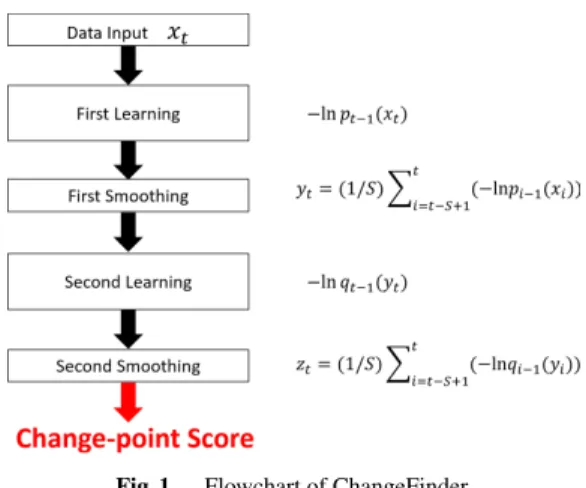
Fig. 1 Flowchart of ChangeFinder
2.2.1 Overview
Figure 1 shows the ChangeFinder algorithm that consists of five steps. Each step is described below.
Step 1 (Data Input)
xtis received at time pointt.
Step 2 (First Learning)
For eacht, an AR model is built. More specifically, a se- quence of probability density functionspt(x) :t=1,2, . . .is obtained by the SDAR model, which will be explained later.
Please note that pt−1is learned based onxt−1. The “outlier”
score atxtis calculated as follows.
S core(xt)=−logpt−1(xt) (4) Step 3 (First Smoothing)
For eacht, a moving average of the outlier scores (obtained in Step 2) in a time window is calculated. More specifi- cally, a sequence of moving averages of the outlier scores yt:t=0,1,2. . .is obtained as follows.
yt= 1 T
t
i=t−T+1
S core(xi), (5)
whereTis the length of a time window.
Steps 4 & 5 (Second Learning & Smoothing)
For eacht, an AR model is built for the new time-series data yt:t=0,1,2, . . . (obtained in Step 3), and a sequence of new probability density functions qt(x) :t=1,2, . . . is ob- tained by the SDAR model as well as Step 2. A smoothing step is also applied as well as Step 3. Thus, a sequence of the moving averageszt:t=0,1,2, . . .is obtained as follows.
zt= 1 T
t
i=t−T+1
(−lnqt−1(yt)) (6)
Here,ztis denoted as the “change-point” score at time
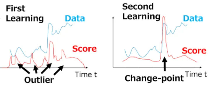
Fig. 2 Two-phase learning of ChangeFinder
t. A higher change-point scoreztindicates a higher possibil- ity of change-point at timet. As shown in Fig. 2, by using the two-phase learning, outliers are eliminated by the first smoothing step and thus only the change-points where the probability distribution of time series changes are extracted.
2.2.2 SDAR Model
SDAR model is used for online discounting learning that relies on AR model. ChangeFinder algorithm uses SDAR model to obtain the sequences of probability density func- tions pt(x) and qt(x). These probability density functions are derived fromωtandΣin Eq. (1). These parameters are updated by following expressions each time.
μˆ :=(1−r) ˆμ+rxt (7)
Cj :=(1−r)Cj+r(xt−μ)(xˆ t−j−μ)ˆ T (8) ˆ
xt :=
k
i=1
ωˆi(xt−i−μ)ˆ +μˆ (9)
Σˆ :=(1−r) ˆΣ +r(xt−xˆt)(xt−xˆt)T (10) Here,ris a discounting rate. A smallerrindicates a greater influence on past data. For eacht, an weighted average ˆμis updated usingrandxtin Eq. (7). Based onCj: j=1, . . . ,k obtained in Eq. (8), estimatedω1, . . . , ωk(denoted as ˆω1, . . ., ωˆk) are derived so that the following equation is satisfied.
k
i=1
ωiCj−i=Cj (11)
Then ˆω1, . . . ,ωˆkare used for Eq. (9).
By introducing the discounting effect, SDAR model can be used for online learning on non-stationary time-series data. In addition, the computation cost is reduced down to O(n) and thus it is preferred for online change-point detec- tion.
2.3 Related Work
In this paper, change-point detection using ChangeFinder algorithm is implemented on an FPGA NIC that has four 10GbE interfaces. NPCUSUM (Non-Parametric Cumula- tive SUM) is a classic and simple change-point detection al- gorithm. In a paper[11], it is implemented on a high-speed FPGA NIC in order to detect attacks from network. The net- work attack detection using NPCUSUM is illustrated below.
S0 =0 (12)
Sn =max{0,Sn−1+Xn−μˆ−θ},ˆ (13) where Xndenotes input data. ˆμis an estimated value ofXn
before an attack, ˆθis that after the attack, and is a tun- ing parameter. An attack from the network is detected when Snbecomes unstable and changes drastically. Although this approach is quite simple to implement, some parameters must be known in advance depending on given applications.
In addition the design presented in the paper[11]achieves 100Gbps when fixed-point values are fed as inputs, while it is 2.5Gbps when floating-point values are fed. Please note that the proposed ChangeFinder NIC can process floating- point inputs at 10Gbps, so it is superior than the paper[11]
in terms of throughput when floating-point values are used in the application.
There are some prior works that present FPGA-based outlier detection that detects anomaly values (not change- points). In a paper[12], for example, an outlier detection based on Mahalanobis distance is implemented in an FPGA NIC. As a more practical outlier detection algorithm, in a paper[13], LOF (Local Outlier Factor) algorithm is ac- celerated by using an FPGA. Normal data are filtered at the NIC and only anomaly data are transferred to the host machine to reduce data size. In addition, KNN (K-Nearest Neighbor) algorithm is accelerated by using FPGAs in pa- pers[13],[14]. It can be used for outlier detection on time- series data. LetXtdenote input data at timet. Among recent data,knearest neighbors fromXtare extracted by KNN al- gorithm. If their average distance from Xtexceeds a given threshold, thenXtis detected as an outlier.
In this paper, the proposed system can find change- points on multiple streams coming from a 10GbE interface.
In other words, we assume multiple time-series data (or mul- tiple streams) which are independent but coming from the same interface. The design highly depends on whether com- putation result of a single sample is influenced by the previ- ous samples in the same stream. If it is not influenced by the previous samples in the same stream, an incoming sample is simply processed without considering the previous com- putation result of the same stream; thus a context for each stream is not considered.
On the other hand, if a computation result is influenced by the previous samples in the same stream, a context must be maintained for each stream. A straightforward approach for such cases is to increase the number of stream processing cores so that each core is in charge of a single stream. In this case, workload can be distributed to multiple cores. In a pa- per[15], an FPGA-based FFT processing for variable length and multiple streams is proposed by using this method. In a paper[16], a compression mechanism for floating-point nu- merical data streams is proposed by using FPGA. In these cases, multiple instances are introduced to handle multiple streams. The number of instances should be carefully se- lected by considering the expected number of streams.
Another approach is to handle multiple streams using a single instance. In this case, a context for each stream
is maintained, and it is switched depending on the sample data currently being processed. For the context switching, a context of the current stream is stored and then that of the next stream is loaded. In papers[17],[18], a regular ex- pression matching mechanism for virus detection is imple- mented by using FPGA, and context memories for storing context data to support multiple streams are implemented by using distributed RAMs or external memory. In this paper, we employ this approach to find change-points on multiple streams.
Although our target is change-point detection to detect trend changes, ChangeFinder algorithm can be used for both the change-point detection and outlier detection. Actually, the result of the first learning phaseS core(xt) is used as outlier score, while the final output zt is used as change- point score. Please note that this paper is the first work that accelerates ChangeFinder algorithm that supports both the change-point and outlier detections by using FPGA NIC.
3. ChangeFinder on FPGA
ChangeFinder module on FPGA is illustrated in this section.
It is integrated into an FPGA NIC in Sect. 4. ChangeFinder module is written in C. As a high-level synthesis tool we use Xilinx Vivado HLS for the implementation.
3.1 Pipeline Structure
Figure 3 illustrates an overview of ChangeFinder module.
It consists of pipelined six stages as mentioned in Sect. 2.2.
As input data, a 32-bit float value is fed to the module. It is processed as follows.
• sdar1: A probability density function pt(x) for input dataxtin the first learning phase is computed.
• log1: A logarithmic loss of the probability density function is computed as an outlier score.
• smooth1: A moving averageytof the outlier scores is computed as a result of the first learning phase.
• sdar2: A probability density functionqt(x) forytin the second learning phase is computed.
• log2: A logarithmic loss of the probability density function is computed as a log loss score.
• smooth2: A moving averageztof the log loss scores is computed as a change-point score.
These stages operate at 125MHz. In Fig. 3, the num- ber in each pipeline stage indicates the minimum interval between two input data in the stage. For example, “1clk” in- dicates that new data can be accepted in every cycle. Thus, log1,smooth1,log2, andsmooth2can accept new data every cycle, whilesdar1andsdar2accept new data in every eight cycles. Please note thatsdar1 andsdar2, log1 andlog2, andsmooth1andsmooth2are identical, respectively. Each module is pipelined by the HLS PIPELINE directive. The input interval values in Fig. 3 represent the values obtained by this pipelining. Also, the memory in each module is op- timized by the HLS ARRAY PARTITION directive. The
Fig. 3 Pipeline of ChangeFinder module
Fig. 4 sdarmodule
input interval ofsdar1andsdar2modules is currently eight cycles. This is becauseupdate omegasubmodule ofsdar1 andsdar2modules takes eight cycles to process each input data. Further optimization of the input interval is our future work. In the following,sdar1,log1, andsmooth1modules are illustrated.
3.2 SDAR Module
Figure 4 showssdarmodule. Its inputs are rand xt. ris a discounting parameter. Based on it, (1−r) is computed.
xtis an input float value. The outputs are ˆxand ˆΣ. ˆxis an estimated value ofxtand ˆΣis that ofΣt.
As shown,sdar1is further divided into five pipelined submodules: update mu, update c, update omega, up- date estx, andupdate sigma. xt is stored in (k+1) 32-bit registers (pastData in the figure) to refer to pastkdata, where kis the order of AR model. Similarly,Ciandωiare accu- mulated in (k+1) 32-bit registers, respectively.
xt,r, and (1−r) are fed toupdate musubmodule. It is corresponding to Eq. (7) and computesμ.μis then fed toup- date candupdate estxsubmodules.update csubmodule is corresponding to Eq. (8) and updatesCiregisters. Using the updatedCiregisters, update omegasubmodule updates ωi
registers based on Eq. (11). update estxsubmodule is cor- responding to Eq. (9). Using the updatedωiregisters, past- Data registers, andμ, it computes ˆxt. Finally,update sigma
submodule is corresponding to Eq. (10). Using ˆxtandxt, it computes ˆΣ.
These five submodules work in a pipelined manner. As a result, sdar1module accepts new data xt in every eight cycles.
3.3 Log and Smooth Modules
Regardinglog1module, its inputs are ˆxt, ˆΣ, andxtin a 32- bit float format. The 32-bit output is used as an outlier score (forlog2, it is used as a log loss score). It performs a log- arithmic computation as in Eq. (4). It is fully pipelined and can accept new data in every cycle.
Regarding smooth1 module, its inputs are a window sizeT and the 32-bit outlier score from log1 module (for smooth2, it is the 32-bit log loss score fromlog2module).
The 32-bit output is the result of the first learning phaseyt
(for smooth2, it is the change-point score zt). The input score is stored in (T +1) 32-bit registers to refer to past Tdata. Then it computes a moving average of recentTdata as in Eq. (5). The maximumT is set to eight in our design.
It is also fully pipelined and can accept new data in every cycle.
4. ChangeFinder on FPGA NIC
ChangeFinder module is implemented on a 10GbE FPGA NIC. It is denoted as ChangeFinder NIC in this paper. It performs change-point detection for each numerical value coming from the 10GbE network. The change-point score computed at the NIC is passed to a host application so that it can identify changes in given time series data. Users can give some parameters (i.e., AR model orderk, discounting rater, and smoothing window sizeT) to the ChangeFinder NIC viaioctlso that the users can tune ChangeFinder mod- ule suitable for time series data of the target application.
In this paper, NetFPGA-SUME[19] is adopted as a 10GbE FPGA NIC. It has four 10GbE interfaces. Pack- ets received by these interfaces are processed at an on-board FPGA and the results are transferred to a host machine via a PCI-Express Gen3 x8 interface. We use 10GbE MAC IP core provided by Xilinx. We also use Reference NIC de- sign provided by NetFPGA project[20]as a standard 10GbE NIC function. ChangeFinder module is inserted along the datapath of Reference NIC design.
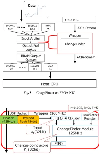
We implemented a wrapper module along the datap- ath of Reference NIC design so that all the received packets go through the wrapper module. Then ChangeFinder mod- ule designed with Xilinx Vivado HLS is implemented inside the wrapper module. Figure 5 shows a block diagram of ChangeFinder NIC consisting of ChangeFinder module and Reference NIC. In Reference NIC, packets received by the four 10GbE interfaces (i.e., RX0 to RX3) and host DMAC are arbitrated at Input Arbiter module. Then, an output port is selected among the four 10GbE interfaces (i.e., TX0 to TX3) and host DMAC for each packet. Packets are stored and transmitted via BRAM Output Queues corresponding
Fig. 5 ChageFinder on FPGA NIC
Fig. 6 Connection between wrapper and ChangeFinder modules
to the selected output ports. Packets are transferred between these modules as AXI4 stream[21]. The wrapper module is implemented between Input Arbiter and Outport Lookup modules. We use UDP/IP as transport/network layer proto- cols. ChangeFinder module computes a change-point score for each incoming packet destined to a specific UDP port.
All the other packets including ARP and ICMP just skip the wrapper module without any additional delay.
Figure 6 illustrates the wrapper module and in- put/output signals of ChangeFinder module. Their con- nection complies with AXI4 standard. A clock generator of 125MHz and parameter registers are implemented for ChangeFinder module. In addition, an input asynchronous FIFO buffer is inserted between them. Because Change- Finder module is operating at 125MHz and Reference NIC is operating at 160MHz, the input FIFO buffer is used to absorb their different clock frequencies.
The wrapper module identifies packets that contain sample data. Then it extracts the sample data and feeds them to ChangeFinder module. The packet conveys sample data xt in a 32-bit float format in a UDP payload. UDP pack- ets with a specific destination port number are extracted as sample packets and they are fed to the input FIFO buffer.
As tuning parameters, AR model orderk, discounting rate
r, and smoothing window sizeTare stored in the parameter registers. They are fed to ChangeFinder module in addition to input dataxtwhen ChangeFinder module is ready. Then the change-point scoreztis computed and fed to an output asynchronous FIFO buffer. The scoreztcan be embedded in the original packet and passed to host application. It is also stored in a register inside the wrapper module which can be accessed by the host application viaioctl.
5. Extension for Multiple Streams
ChangeFinder module illustrated so far is designed to find change-points on a single stream. In this section, it is ex- tended to support multiple streams coming from a 10GbE interface. Actually, it is practical to assume that multiple streams from one or more sources are fed to the proposed ChangeFinder NIC. We are assuming some applications for this implementation, such as a server that aggregates sensor values from many sensor nodes. It can be applied to an in- trusion detection system that monitors many network flows between host and specific IP addresses. The change-point detection requires a context for each stream, because com- putation result of a sample is influenced by the previous re- sults in the same stream. As discussed in Sect. 2, a straight- forward design is to replicate the ChangeFinder module so that each module is in charge of a single stream. However, as shown in Sect. 6.3, the number of instances which can be implemented on the FPGA NIC is at most eight, while the number of streams can be easily increased depending on the number of stream sources. In this section, we thus extend the ChangeFinder module so that a single instance can sup- port multiple streams by using a context memory to store context of each stream.
In our design, a fine-grained context switching, where a context switching occurs in each pipeline stage separately, is implemented. Such a fine-grained context switching is beneficial compared to the “Run-to-Completion” approach, where context of all the pipeline stages is switched at the same time, in terms of context switching latency. Figure 7 shows the multi-stream version assumingk=2 andT =8.
There are a BRAM-based context memory and six stages:
sdar1,log1,smooth1,sdar2,log2, andsmooth2.
Each stage identifies the stream ID of the sample cur- rently being processed. It loads and saves the necessary context from/to the context memory based on the stream ID currently being processed. That is, the stream ID is used as address of the context memory.
Context data for all the streams must be maintained, while the number of streams can be easily increased depend- ing on the number of stream sources; thus context data size should be minimized. Context data size depends on the or- der of AR modelkand the smoothing window sizeT. Ta- ble 1 lists context data fields and their sizes whenk = 2 andT = 8. In this case, the context size for each stream is 76 bytes. Assuming Xilinx Virtex-7 XC7VX690T FPGA is used for the implementation, because its BRAM capacity is about 52.9 Mbits, up to 87,006 streams can be stored in
Fig. 7 ChangeFinder module for multiple streams
Table 1 Context data for each stream
Data Ci Σ pastData μ r ω index count
Size (byte) 12 4 32 4 4 12 4 4
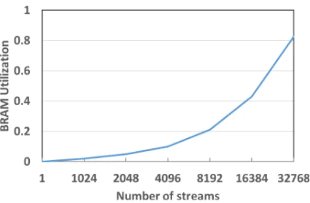
the BRAM. Please note that only 32,768 streams could be implemented in total after the placement and routing were done. This is because the NIC part also consumes BRAM.
If the number of streams is less than the BRAM capacity, a fast context switching can be simply implemented without any external memories.
6. Evaluations
6.1 Preliminary Evaluations of Parameters
Context data size depends on the order of AR modelkand the smoothing window sizeT, so we conduct two prelimi- nary evaluations using real datasets in order to find appro- priate parameters of ChangeFinder.
First we apply ChangeFinder to a network intrusion de- tection. We use CICIDS2017 dataset[22]provided by Uni- versity of New Brunswick. This dataset consists of labeled network flows during five days. We use Wednesday dataset which includes various DDoS attacks, because papers[8]
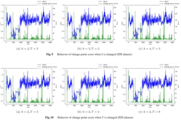
and[23]show that detection of DDoS attack is one of appli- cations for their change-point detection algorithm. The rate of SYN flag and FIN flag which is updated every second is used as input for ChangeFinder.ris set to 0.001. The eval- uation results while changingkandT are shown in Figs. 9 and 10.
Figure 9 shows the result whenkis changed to 2, 3, and 4 while T is fixed to 3. The blue line represents the input value, and the green line represents the change-point score. X-axis shows the elapsed time and the time unit is one second. The result shows that the point at which the change-point score becomes high is almost the same in these kvalues, and it is not necessary to setklarger than 2 for this dataset.
Figure 10 shows the result whenT is changed to 3, 4, and 8 whilekis fixed to 2. SinceT is the smooth window size, the change-point score decreases asT increases.
Secondly we apply ChangeFinder to analyze stock data. We use TOPIX (Tokyo stock price index) data[24]
Fig. 9 Behavior of change-point score whenkis changed (IDS dataset)
Fig. 10 Behavior of change-point score whenTis changed (IDS dataset)
from 1987 to 2019.ris set to 0.005. The evaluation results while changingkandTare shown in Figs. 11 and 12. X-axis shows the elapsed time and the time unit is one day.
As far as the two evaluation results are considered, it can be said thatkis enough high even at around 2. On the other hand,T depends on the sensibility of the input value and how much the change is ignored as an outlier. There was no significant differences in the number of change points in these evaluations. Please note that the maximumT must be determined when ChangeFinder core is synthesized. In the current implementation, the maximumTis set to 8 which is the largest value confirmed in the preliminary evaluations.
6.2 Evaluation Environment
The target 10GbE FPGA NIC is NetFPGA-SUME that has a Xilinx Virtex-7 XC7VX690T FPGA and four SFP+10GbE interfaces. It is mounted to a host machine via PCI-Express Gen3 x8 interface. We use Xilinx Vivado HLS version 2016.4 for the implementation. Reference NIC part is oper- ating at 160MHz, while the proposed ChangeFinder module is running at 125MHz in the case of single-stream design.
Figure 8 shows the evaluation environment using two machines and Table 2 shows their specification. In the throughput measurement, if a software program at the client machine generates time series data and sends them to the server, there is a possibility that the client cannot fully uti-
Fig. 8 Evaluation environment for throughput
Table 2 Machines used in the environment Server (host) machine Client machine CPU Intel Core i5-4460 Intel Core i5-4460
OS Ubuntu 14.04 CentOS 6.6
NIC NetFPGA-SUME (Proposal) NetFPGA-10G for OSNT Intel X520-DA2 (Software)
lize the 10GbE bandwidth. Therefore, we used a hard- ware packet generator, called Open Source Network Tester (OSNT), as the client. OSNT is implemented on the FPGA NIC and can generate packets at the throughput of 10GbE line rate. The client and server machines are connected by a SFP+direct attached cable for 10GbE. The client machine has an FPGA NIC with OSNT installed, and sends packets to the server. In the server machine, the proposed Change- Finder module is implemented on the FPGA NIC and pro-
Fig. 11 Behavior of change-point score whenkis changed (TOPIX dataset)
Fig. 12 Behavior of change-point score whenTis changed (TOPIX dataset)
cesses incoming time series data. We measured the number of sample data processed at the ChangeFinder module per a second as throughput.
6.3 Resource Utilization
In this section, first, ChangeFinder module for a single stream is evaluated in terms of resource utilization. That for multiple streams is then evaluated.
Table 3 shows DSP, FF, and LUT utilizations of sub- modules (i.e., sdar1, log1, smooth1, sdar2, log2, and smooth2) in the proposed ChangeFinder module for a sin- gle stream. Table 4 shows those of whole ChangeFinder NIC including ChangeFinder module and Reference NIC.
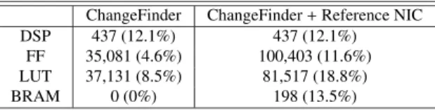
Althoughlog1andlog2submodules that perform logarithm computations in parallel consume more resources than the others, their resource utilizations are still low. As shown in Table 4, ChangeFinder module consumes up to 12.1% of the FPGA resources. Even with 10GbE NIC functionality, the entire resource utilizations are less than or equal to 18.8%.
Regarding the processing time, it takes 347 cycles to com- plete all the processing for a single sample, so the latency of all the processing is 2.78μsec.
Although up to eight ChangeFinder modules can be im- plemented on the FPGA according to Table 4, in this pa- per, as shown in Sect. 5, we do not increase the number of ChangeFinder modules but increase the capacity of a single
Table 3 Resources used in single-stream ChangeFinder module sdar1 log1 smooth1 sdar2 log2 smooth2
DSP 39 122 14 39 122 14
FF 5,426 9,070 2,777 5,426 9,070 2,777
LUT 5,202 11,491 2,864 5,202 11,491 2,864
Table 4 Resources used in single-stream ChangeFinder NIC ChangeFinder ChangeFinder+Reference NIC
DSP 437 (12.1%) 437 (12.1%)
FF 35,081 (4.6%) 100,403 (11.6%) LUT 37,131 (8.5%) 81,517 (18.8%)
BRAM 0 (0%) 198 (13.5%)
ChangeFinder module so that it can support many streams.
In this case, the size of the BRAM-based context mem- ory increases as the maximum number of streams increases.
Figure 13 shows the BRAM utilization when increasing the maximum number of streams. Up to 32,768 streams can be implemented on the BRAM. When increasing the num- ber of streams from one to 32,768, the operating frequency dropped from 125MHz to 80MHz. When 32,768 streams are implemented, the operating frequency is 80MHz and the number of clock cycles to process a single sample is 260, so the processing latency is 3.25μsec, which is 0.47μsec longer than the original design that supports a single stream. Ta- ble 5 shows the resource utilizations of ChangeFinder NIC that supports 32,768 streams.
Fig. 13 BRAM utilization for multiple streams
Table 5 Resources used in multi-stream ChangeFinder NIC ChangeFinder ChangeFinder+Reference NIC
DSP 376 (10.4%) 376 (10.4%)
FF 25,213 (3.3%) 89,659 (10.4%) LUT 36,766 (8.4%) 80,470 (18.6%) BRAM 1,216 (82.7%) 1,414 (96.2%)
BRAM utilization is 96.2%, while the other resource utilizations are less than 18.6%. FF utilization is lower than that of the single-stream design since a part of FFs are re- placed with BRAMs. The other resource utilizations, such as DSP and LUT, are also reduced because of a relaxed tim- ing constraint targeting 80MHz.
6.4 Throughput
As mentioned above, OSNT at the client machine transmits time-series data at 10GbE line rate to the server machine, and the number of sample data processed within one second at the server machine is measured as throughput.
The proposed ChangeFinder NIC is compared with three software-based counterparts implemented in C: Base- line, DPDK, and Netfilter. In Baseline, a ChangeFinder program is running on the application layer. A standard UDP/IP processing is performed by Linux kernel for each sample data. In DPDK, although the ChangeFinder program is running on the application layer, the program directly ac- cesses the NIC without kernel UDP/IP stack. In Netfilter, the ChangeFinder program is implemented as a kernel mod- ule using a Linux Netfilter framework. Please note that a float value is approximated as a fixed-point format in the Netfilter version. In all these cases, a single-stream Change- Finder is used for the measurement.
Figure 14 shows their throughputs. The throughput of our ChangeFinder module is denoted as FPGA(sim) and the ChangeFinder NIC consisting of ChangeFinder and Refer- ence NIC modules is denoted as FPGA(actual). FPGA(sim) throughput is a theoretical value. It is the upper limit of throughput via 10GbE. The throughput of ChangeFinder module itself, which is derived by the number of cycles, pipeline structure (i.e., interval), and operating frequency of the ChangeFinder module, is 15.6M packets per second.
Fig. 14 Throughput of change-point detection [mega samples/sec]
Fig. 15 Packet format for the evaluation of multi-stream
FPGA(actual) is the measured throughput using real ma- chines (Table 2). The throughput of FPGA(actual) achieves 16.8x throughput improvement compared to Baseline. It is much higher than those with software-based optimizations by DPDK and Netfilter. FPGA(actual) and FPGA(sim) are almost the same.
In practical use cases, a specific field of received pack- ets is extracted and fed to ChangeFinder module. In this experiment, we used 46-byte UDP/IP packets containing a single 32-bit float value. This assumption is pessimistic in terms of throughput. sdar1andsdar2modules accept new data in every eight cycles. Since internal data width of Ref- erence NIC is 256 bits, thesesdarmodules are not bottle- neck when packet length is greater than or equal to 256 bytes. Spdenotes the packet length [bits] andSoverhead de- notes the total size [bits] of preamble, FCS, and IFG.Tactual
denotes the throughput [samples/sec] of FPGA(actual). Ra- tio against the 10GbE line rate is denoted as L, and it is calculated as follows.
L=Tactual(Sp+Soverhead)/10G[bits/sec] (14)
The proposed FPGA(actual) achieves 10GbE line rate.
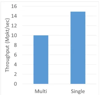
We also evaluate the throughput of the multi-stream implementation by RTL simulation. The packet format pro- cessed in the NIC is shown in Fig. 15. The format includes a float value and a stream ID which is generated randomly.
The throughput was calculated based on the number of clock cycles required to process 10,000 packets. Figure 16 shows their throughputs. Throughput of the multi-stream imple- mentation is sightly lower than the single-stream implemen- tation due to a reduced operating frequency.
7. Conclusions
Toward anomaly detection, change-point detection is used to look for change in a probability distribution of time series, while outlier detection is used to look for entity being away from the mean of a probability distribution.
ChangeFinder algorithm based on SDAR model supports both the outlier and change-point detections and can be used
Fig. 16 Throughput evaluation of multi-stream
for online use. This paper is the first work that acceler- ates ChangeFinder algorithm using FPGA and integrates it into NetFPGA-SUME for high-speed change-point detec- tion at 10GbE NICs. A single ChangeFinder module can find change-points on many streams coming from the same 10GbE interface by using a BRAM-based fast context mem- ory. The proposed ChangeFinder NIC is compared to a UDP baseline and two software-based optimizations, i.e., DPDK and Netfilter. The throughput is much higher than these counterparts and it is 16.8x higher than the UDP baseline.
The throughput is corresponding to the 10GbE line rate. A demonstration video of current design can be found in[25].
Acknowledgments
This work was supported by JST CREST Grant Number JPMJCR1785, Japan.
References
[1] H. Wang, D. Zhang, and K.G. Shin, “Change-Point Monitoring for the Detection of DoS Attacks,” IEEE Trans. Dependable and Secure Computing, vol.1, no.4, pp.193–208, Oct. 2004.
[2] S. Aminikhanghahi and D.J. Cook, “A Survey of Methods for Time Series Change Point Detection,” Knowledge and Information Sys- tems, vol.51, no.2, pp.339–367, May 2017.
[3] V. Guralnik and J. Srivastava, “Event Detection from Time Series Data,” Proc. International Conference on Knowledge Discovery and Data Mining (KDD’99), pp.33–42, Aug. 1999.
[4] J. Takeuchi and K. Yamanishi, “A Unifying Framework for Detect- ing Outliers and Change Points from Time Series,” IEEE Trans.
Knowl. Data Eng., vol.18, no.4, pp.482–492, 2006.
[5] T. Iwata, K. Nakamura, Y. Tokusashi, and H. Matsutani, “Accel- erating Online Change-Point Detection Algorithm using 10 GbE FPGA NIC,” Proc. International European Conference on Parallel and Distributed Computing (Euro-Par’18) Workshops, vol.11339, pp.506–517, Aug. 2018.
[6] Y. Urabe, K. Yamanishi, R. Tomioka, and H. Iwai, “Real-Time Change-Point Detection Using Sequentially Discounting Normal- ized Maximum Likelihood Coding,” Proc. Pacific-Asia Conference
on Knowledge Discovery and Data Mining (PAKDD’11), vol.6635, pp.185–197, May 2011.
[7] Y. Kawahara and M. Sugiyama, “Change-Point Detection in Time-Series Data by Direct Density-Ratio Estimation,” Proc. SIAM International Conference on Data Mining (SDM’09), pp.389–400, April 2009.
[8] K. Yamanishi and J. Takeuchi, “A Unifying Framework for Detect- ing Outliers and Change Points from Non-Stationary Time Series Data,” Proc. International Conference on Knowledge Discovery and Data Mining (KDD’02), pp.676–681, July 2002.
[9] F. Saaid, D. Nur, and R. King, “Change Points Detection of Vector Autoregressive Model using SDVAR Algorithm,” Proc. 5th Annual ASEARC Conference, pp.18–21, Feb. 2012.
[10] “Apache Hivemall.” http://hivemall.incubator.apache.org/. [11] P. Ben´aˇcek, R.B. Blaˇzek, T. ˇCejka, and H. Kub´atov´a, “Change-
Point Detection Method on 100 Gb/s Ethernet Interface,” Proc.
ACM/IEEE Symposium on Architectures for Networking and Com- munications Systems (ANCS’14), pp.245–246, June 2014.
[12] A. Hayashi, Y. Tokusashi, and H. Matsutani, “A Line Rate Out- lier Filtering FPGA NIC using 10GbE Interface,” ACM SIGARCH Computer Architecture News, vol.43, no.4, pp.22–27, Sept. 2015.
[13] A. Hayashi and H. Matsutani, “An FPGA-Based In-NIC Cache Approach for Lazy Learning Outlier Filtering,” Proc. International Conference on Parallel, Distributed, and Network-Based Processing (PDP’17), pp.15–22, March 2017.
[14] Y. Pu, J. Peng, L. Huang, and J. Chen, “An Efficient KNN Al- gorithm Implemented on FPGA Based Heterogeneous Computing System Using OpenCL,” Proc. International Symposium on Field- Programmable Custom Computing Machines (FCCM’15), pp.167–
170, May 2015.
[15] P.P. Boopal, M. Garrido, and O. Gustafsson, “A Reconfigurable FFT Architecture for Variable-Length and Multi-Streaming OFDM Stan- dards,” Proc. International Symposium on Circuits and Systems (IS- CAS’13), pp.2066–2070, May 2013.
[16] T. Ueno, K. Sano, and S. Yamamoto, “Bandwidth Compression of Floating-Point Numerical Data Streams for FPGA-Based High- Performance Computing,” ACM Trans. Reconfigurable Technol.
Syst., vol.10, no.3, pp.18:1–18:22, May 2017.
[17] Q. Yun, Y.-H.E. Yang, and V.K. Prasanna, “Multi-Stream Regular Expression Matching on FPGA,” Proc. International Conference on Reconfigurable Computing and FPGAs (ReConFig’11), pp.86–91, Nov. 2011.
[18] Y. Qu, Y.-H.E. Yang, and V.K. Prasanna, “Large-Scale Multi-Flow Regular Expression Matching on FPGA,” Proc. International Con- ference on High Performance Switching and Routing (HPSR’12), pp.70–75, June 2012.
[19] N. Zilberman, Y. Audzevich, G.A. Covington, and A.W. Moore,
“NetFPGA SUME: Toward 100 Gbps as Research Commodity,”
IEEE Micro, vol.34, no.5, pp.32–41, Sept. 2014.
[20] “The NetFPGA Project.” http://netfpga.org/. [21] Xilinx, AXI Reference Guide, 2011.
[22] I. Sharafaldin, A.H. Lashkari, and A.A. Ghorbani, “Toward Generat- ing a New Intrusion Detection Dataset and Intrusion Traffic Charac- terization,” Proc. 4th International Conference on Information Sys- tems Security and Privacy, pp.108–116, 2018.
[23] A.G. Tartakovsky, B.L. Rozovskii, R.B. Blazek, and H. Kim, “A novel approach to detection of intrusions in computer networks via adaptive sequential and batch-sequential change-point detection methods,” IEEE Trans. Signal Process., vol.54, no.9, pp.3372–3382, 2006.
[24] “TOPIX historial price.” https://quotes.wsj.com/index/JP/XTKS/ I0000/historical-prices.
[25] YouTube, “Accelerating ChangeFinder using 10Gbps FPGA NIC.”
https://www.youtube.com/watch?v=wgTcBfkE5hY.
Takuma Iwata received the BE degree from Keio University in 2018. He is currently a mas- ter course student in Keio University.
Kohei Nakamura received the BE and ME degrees from Keio University in 2016 and 2018, respectively.
Yuta Tokusashi received the BA, ME and PhD degrees from Keio University in 2014, 2016, 2019, respectively. He is currently a re- search associate at the Computer Laboratory in the University of Cambridge. His current re- search interests include computer architecture and FPGA systems.
Hiroki Matsutani received the BA, ME, and PhD degrees from Keio University in 2004, 2006, and 2008, respectively. He is currently an associate professor in the Department of Infor- mation and Computer Science, Keio University.
His research interests include the areas of com- puter architecture and interconnection networks.