Which Replacement Is Better at Working Cycles or Number of Failures

PAPER

Which Replacement Is Better at Working Cycles or Number of Failures

Satoshi MIZUTANI^†a),Member, Xufeng ZHAO^††b),Nonmember,andToshio NAKAGAWA^†c),Member

SUMMARY When a unit repeats some works over again and undergoes minimal repairs at failures, it is more practical to replace it preventively at the end of working cycles or at its failure times. In this case, it would be an interesting problem to know which is better to replace the unit at a num- ber of working cycles or at random failures from the point of cost. For this purpose, we give models of the expected cost rates for the following replacement policies: (1) The unit is replaced at a working cycleNand at a failure numberK, respectively; (2) Replacement first and last policies with working cycleNand failure numberK, respectively; (3) Replacement overtime policies with working cycleNand failure numberK, respectively.

Optimizations and comparisons of the policies forNandKare made ana- lytically and numerically.

key words: replacement policies, minimal repair, working cycle, replace- ment last, replacement overtime

1. Introduction

It has become an important problem to plan good mainte- nance policies for a large-scale system such as a plant equip- ment and an information system with network, as they have been widely used in various environments and their sudden failures might incur great losses or even social confusions.

There have been many research works regarding to preven- tive maintenance policies in theory [1]–[4]; however, the difficulties are which maintenance policies are better from the points of cost, practicality and reliability. Further, if we could rank the maintenance policies as needed, but will this rank change when the maintenance environment changes. In order to answer the above questions, this paper tries to give some comparisons of replacement policies when an operat- ing unit is replaced at working cycles or at random failures.

In general, it would be impossible to do some main- tenance during the interval when the unit is operating for works, and it would be better to do maintenance when the work completes or when the unit fails. The theoretical mod- els have shown that maintaining a unit after it completes some works are possible even though they are sometimes costly [5]. The properties of replacement times between two successive failed units were investigated for a system

Manuscript received April 4, 2019.

Manuscript revised July 17, 2019.

†The authors are with Department of Business Administration, Aichi Institute of Technology, Toyota-shi, 470-0392 Japan.

††The author is with College of Economics and Management, Nanjing University of Aeronautics and Astronautics, NO. 29, Jiangjun Avenue, Nanjing 211106, China.

a) E-mail: [email protected] b) E-mail: [email protected] c) E-mail: [email protected]

DOI: 10.1587/transfun.2019EAP1049

which replaced only at random times [6]. Several random and age replacement models were discussed[7]for an op- erating unit which repeats some works over again. The maintenance model with age T and number of jobs com- pletedNhas been considered[8]. Considering the systems successively executing jobs with random working times, it would be better to conduct the maintenance after the jobs completed. Other maintenance models with random work- ing cycle have been studied extensively [9]–[11]. Further- more, replacement first and last with two kinds of failures were considered and their optimal policies were discussed and compared[12]. Replacement policies in which a main- tainer made the postponed replacement in a delay time due to inspection test were studied[13].

Nakagawa and Zhao considered about first and last policies for replacement and inspections when the policies are triggered by two factors. [14]–[16]. Replacement first means that the unit is replaced preventively at time of events such as operating time, number of repairs, working cycles, cumulative damage, etc, whichever occurs first, andreplace- ment lastmeans that the unit is replaced preventively at the above events, whichever occurs last. It has been shown that[15]replacement last policies could let the unit operate works as longer as possible while replacement first polices are more easily to save total maintenance cost. Replacement first and last polices are good alternatives when the unit per- forms one big project and the decision on replacement is based on the termination time of the project[10].

For replacement first and last policies, it is an interest- ing problem to determine which policies are better from the points of cost, practicality and reliability. The recent work [17]has given some comparative methods for replacement policies when they are performed at continuous or discrete times. However, when the unit can be only replaced pre- ventively at discrete times such as working cycles or at ran- dom failures, this paper will answer the questions like how we can formulate the replacement first and last policies, and how we can know which policy is better from the point of cost. For this purpose, the following policies are given: (1) The unit is replaced at theNth (N =1,2, . . .) working cy- cle, and theKth (K=1,2, . . .) failure, respectively; (2) the unit is replaced at theNth working cycle or theKth failure, whichever occurs first and last. In addition, it is a possi- ble way to delay the replacement policies over a planned time, whose models are called replacement overtime[18], so that the above policies are extended to overtime replace- ment policies with working cyclesNand failuresK.

Copyright c2020 The Institute of Electronics, Information and Communication Engineers

524

We formulate the expected cost rates, give analytical discussions and make comparisons to decided which is bet- ter for the above replacement policies in each sections. Fi- nally, we give the properties of extended failure rates which are needed for theoretical analysis of optimal policies in Ap- pendix.

2. Assumptions

We give the following assumptions for the models in this paper:

1. The unit repeats some works over again which have random working cyclesYj(j=1,2, . . .). It is assumed thatYjare independent and identically distributed ran- dom variables and have an identical distributionG(t)≡ Pr{Yj ≤ t}with finite mean 1/θ ≡ R∞

0 G(t)dt, where G(t) ≡1−G(t). LetG⁽ⁿ⁾(t) (n =1,2, . . .) denote the n-fold Stieltjes convolution ofG(t) andG⁽⁰⁾(t)≡1 for t≥0.

2. It is assumed that failures occur in a nonhomogeneous Poisson process withH(t) ≡ Rt

0h(u)du. Let pj(t) de- note the probability that the number of failures in [0,t]

is j, i.e.,

pj(t)≡ H(t)^j

j! e^−H(t) (j=0,1,2, . . .). (1) We assume that the failure rate h(t) increases strictly fromh(0) = 0 toh(∞) = ∞for simplicity of discus- sions.

3. LetPK(t) ≡ P∞

j=Kpj(t) and PK(t) ≡ PK−1

j=0 pj(t) (K = 0,1,2, . . .), where note thatP−1

j=0 ≡0. Further, we have the following relations fort (0 < t < ∞) and j (j = 0,1,2, . . .),

P_j+1(t)=Z t 0

p_j(u)h(u)du, Pj+1(t)=Z ∞

t

pj(u)h(u)du, Z ∞ 0

pj(t)h(t)dt=1, Z ∞

0

H(t)dPj(t)=Z ∞ 0

Pj(t)h(t)dt

=

j−1

X

i=0

Z ∞

0

pi(t)h(t)dt= j.

4. The probability that some failures occur in (0,t] is given byF(t) ≡ P∞

j=1p_j(t) = 1−p0(t) = 1−e^−H(t) with finite meanµ, andf(t) is a density function ofF(t) and f(t) ≡ dF(t)/dt. Thus, for given t(0 ≤ t < ∞), the probability that a failure occurs in (u,u +du] is

f(u)du/F(t) foru>t.

5. When the failure has occurred, the unit is replaced or undergoesminimal repair. The unit after minimal re- pair has the same failure rate as before rate[3, p. 96].

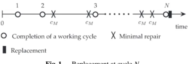
Fig. 1 Replacement at cycleN.

3. Basic Policies

3.1 Replacement at CycleN

Suppose that the unit is replaced at working cycle N(N = 1,2, . . .) (see Fig. 1). Then, the expected cost rate is [5, p. 76],

C(N)=cN+cM

R∞

0 [1−G^(N)(t)]h(t)dt

N/θ (N=1,2, . . .), (2) where cN = replacement cost at cycleN and cM = cost of minimal repair at each failure.

We find optimal N^∗ to minimizeC(N). Forming the inequalityC(N+1)−C(N)≥0,

Z ∞

0

[1−G^(N)(t)][Q₁(N)−h(t)]dt≥ cN

cM

, (3)

where for 0<T ≤ ∞andN=0,1,2, . . ., Q1(N;T)≡

RT

0 [G^(N)(t)−G^(N+1)(t)]h(t)dt RT

0 [G^(N)(t)−G^(N+1)(t)]dt

≤h(T), Q1(N)≡ lim

T→∞Q1(N;T)

=θZ ∞ 0

[G^(N)(t)−G^(N+1)(t)]h(t)dt.

In particular, whenG(t)=1−e^−θt, Q1(N)=Z ∞

0

θ(θt)^N

N! e^−θth(t)dt,

which increases strictly with N to ∞ from Appendix A.

Thus, there exists a finite and unique minimum N^∗ (1 ≤ N^∗ < ∞) which satisfies (3), and the resulting cost rate is

c_MQ1(N^∗−1)<C(N^∗)≤c_MQ1(N^∗). (4)

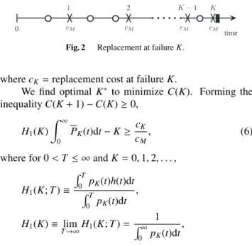
3.2 Replacement at FailureK

Suppose that the unit is replaced at failureK(K=1,2, . . .) (see Fig. 2). Then, the expected cost rate is[3, p. 106]

C(K)= cK+cMK R∞

0 PK(t)dt (K=1,2, . . .), (5)

Fig. 2 Replacement at failureK.

wherecK=replacement cost at failureK.

We find optimalK^∗ to minimizeC(K). Forming the inequalityC(K+1)−C(K)≥0,

H₁(K) Z ∞

0

P_K(t)dt−K≥ cK

cM

, (6)

where for 0<T ≤ ∞andK=0,1,2, . . ., H₁(K;T)≡

RT

0 p_K(t)h(t)dt RT

0 pK(t)dt , H1(K)≡ lim

T→∞H1(K;T)= 1 R∞

0 pK(t)dt,

which increases strictly withKtoh(∞) from Appendix B.

Thus, because the left-hand side of (6) increases strictly with K to∞, there exists a finite and unique minimumK^∗ (1 ≤ K^∗<∞) which satisfies (6), and the resulting cost rate is

c_MH₁(K^∗−1)<C(K^∗)≤c_MH₁(K^∗). (7) 3.3 Numerical Examples

We compute numerically optimalN^∗ andK^∗ whenG(t) = 1−e^−tandH(t)=(λt)², i.e.,h(t)=2λ²t. In this case,

Q₁(N)=Z ∞ 0

t^N

N!e^−t2λ²tdt=2λ²(N+1),

N−1

X

j=0

Z ∞

0

t^j

j!e^−t2λ²tdt=λ²N(N+1), and from (3), optimalN^∗is given by

2λ²N(N+1)−λ²N(N+1)=λ²N(N+1)≥ cN

cM

, (8)

and from (2), C(N^∗)

c_M =cN/cM+λ²N^∗(N^∗+1)

N^∗ . (9)

Further, we can see that Z ∞

0

pK(t)dt=Z ∞ 0

(λt)^2K

K! e^−(λt)2dt= 1 2λ

Γ(K+1/2) Γ(K+1) ,

K−1

X

j=0

Z ∞

0

pj(t)dt= 1 λ

Γ(K+1/2) Γ(K) , and from (6), optimalK^∗is given by

2Γ(K+1/2)/Γ(K)

Γ(K+1/2)/Γ(K+1)−K=K≥ cK

cM

, (10)

Table 1 OptimalN^∗,K^∗,C(K^∗)/cMandC(N^∗)/cMwhenG(t)=1−e^−t, H(t)=(λt)²andc_N=c_K.

λ=0.1 λ=1

c_N

c_M K^∗ N^{∗ C(K}_c ^∗)

M

C(N^∗)

c_M N^{∗ C(K}_c ^∗)

M

C(N^∗) c_M

1 1 10 0.226 0.210 1 2.257 3.000

2 2 14 0.301 0.293 1 3.009 4.000

3 3 17 0.361 0.357 2 3.611 4.500

4 4 20 0.413 0.410 2 4.127 5.000

5 5 22 0.459 0.457 2 4.585 5.500

6 6 22 0.500 0.503 2 5.002 6.000

7 7 24 0.539 0.542 3 5.387 6.333

8 8 26 0.575 0.578 3 5.746 6.667

9 9 28 0.608 0.611 3 6.084 7.000

10 10 32 0.640 0.643 3 6.404 7.333

whereΓ(α)≡R∞

0 x^α−1e^−xdxforα >0. Thus, ifc_K/c_Mis an integer thenK^∗=cK/cM, and from (5),

C(K^∗) cM

= c_K/c_M+K^∗

Γ(K^∗+1/2)/[λΓ(K^∗)]. (11) Table 1 gives optimalK^∗,N^∗,C(K^∗)/cMandC(N^∗)/cM

forλ=0.1, 1, andc_N/c_M=1,2, . . .10. We can see that for λ=1,C(K^∗)/cM<C(N^∗)/cM, that is, replacement withK^∗ is better than replacement withN^∗. On the other hand, for λ =0.1,C(K^∗)/cM >C(N^∗)/cM forK^∗ =cN/cM ≤5, and C(K^∗)/c_M <C(N^∗)/c_Mfor K^∗ ≥6. OptimalN^∗decreases withλ. The reason would be that whenλis large, interval times of failures become small and we should replace early to avoid the cost of failures.

4. Replacement First and Last

4.1 Replacement First

The unit is replaced at cycle N (N = 1,2, . . .) or fail- ure K (K = 1,2, . . .), whichever occurs first (see Fig. 3).

The probability that the unit is replaced at cycle N is R∞

0 PK(t)dG^(N)(t), and the probability that it is replaced at failureKisR∞

0 [1−G^(N)]dP_K(t). The mean time to replace- ment is

Z ∞

0

t PK(t)dG^(N)(t)+Z ∞ 0

t[1−G^(N)(t)]dPK(t)

=Z ∞ 0

[1−G^(N)(t)]P_K(t)dt, (12) and the expected number of failures until replacement is

Z ∞

0

H(t)P_K(t)dG^(N)(t)+Z ∞ 0

H(t)[1−G^(N)(t)]dP_K(t)

=Z ∞ 0

[1−G^(N)(t)]PK(t)h(t)dt. (13) Therefore, the expected cost rate is

CF(N,K)=

cK−(c_K−cN)R∞

0 PK(t)dG^(N)(t) +cM

R∞

0 [1−G^(N)(t)]PK(t)h(t)dt R∞

0 [1−G^(N)(t)]PK(t)dt . (14)

526

Fig. 3 Replacement first withNandK.

Clearly,C_F(∞,K) =C(K) in (5) andC_F(N,∞) =C(N) in (2).

We find optimal N^∗_F and K^∗_F to minimize CF(N,K) whencK = cN andG(t) = 1−e^−θt. Forming the inequal- ityCF(N+1,K)−CF(N,K)≥0,

Q2(N,K) Z ∞

0

[1−G^(N)(t)]PK(t)dt

− Z ∞

0

[1−G^(N)(t)]PK(t)h(t)dt≥ cN

c_M, (15) where

Q2(N,K)≡ PK−1

j=0

R∞

0 (θt)^Ne^−θtpj(t)h(t)dt PK−1

j=0

R∞

0 (θt)^Ne^−θtpj(t)dt ,

which increases strictly withN fromQ2(0,K) toh(∞) and increases strictly withKfromQ2(N,1) to

Q2(N,∞)=Z ∞ 0

θ(θt)^N

N! e^−θth(t)dt=Q1(N)

from Appendix A. Thus, because the left-hand side of (13) increases strictly withNto∞, there exists a finite and unique minimum N^∗_F (1 ≤ N_F^∗ < ∞) which satisfies (15), and the resulting cost rate is

c_MQ₂(N_F^∗−1,K)<C_F(N^∗_F,K)≤c_MQ₂(N_F^∗,K). (16) In addition, noting that the left-hand side of (15) goes to that of (3) asK → ∞,N_F^∗ approaches toN^∗given in (3) asK→ ∞.

Forming the inequalityCF(N,K+1)−CF(N,K)≥0, H2(K,N)

Z ∞

0

[1−G^(N)(t)]P_K(t)dt

− Z ∞

0

[1−G^(N)(t)]P_K(t)h(t)dt≥ c_N cM

, (17)

where

H₂(K,N)≡ PN−1

j=0

R∞

0 [(θt)^j/j!]e^−θtpK(t)h(t)dt PN−1

j=0

R∞

0 [(θt)^j/j!]e^−θtp_K(t)dt , which increases strictly withNfromH2(K,1) to

H2(K,∞)= R∞

0 pK(t)h(t)dt R∞

0 pK(t)dt =H1(K),

and increases strictly withK from H2(0,N) to h(∞) from

Fig. 4 Replacement last withNandK.

Appendix B. Thus, because the left-hand side of (17) in- creases strictly withKto∞, there exists a finite and unique minimum K_F^∗ (1 ≤ K_F^∗ < ∞) which satisfies (17), and the resulting cost rate is

c_MH₂(K_F^∗−1,N)<C_F(N,K^∗_F)≤c_MH₂(K_F^∗,N). (18) In addition, noting that the left-hand side of (17) goes to that of (6) asN → ∞,K_F^∗ approaches toK^∗given in (6) asN→ ∞.

4.2 Replacement Last

The unit is replaced at cycle N (N = 0,1,2, . . .) or fail- ure K(K =0,1,2, . . .), whichever occurs last (see Fig. 4).

The probability that the unit is replaced at cycle N is R∞

0 PK(t)dG^(N)(t) and the probability that it is replaced at failure K is R∞

0 G^(N)(t)dPK(t). The mean time to replace- ment is

Z ∞

0

tPK(t)dG^(N)(t)+Z ∞ 0

t G^(N)(t)dPK(t)

=Z ∞ 0

[1−G^(N)(t)PK(t)]dt, (19) and the expected number of failures until replacement is

Z ∞

0

H(t)PK(t)dG^(N)(t)+Z ∞ 0

H(t)G^(N)(t)dPK(t)

=Z ∞ 0

[1−G^(N)(t)PK(t)]h(t)dt. (20) Therefore, the expected cost rate is

CL(N,K)=

cK−(cN−cK)R∞

0 PK(t)dG^(N)(t) +cM

R∞

0 [1−G^(N)(t)PK(t)]h(t)dt R∞

0 [1−G^(N)(t)PK(t)]dt . (21) Clearly,CL(0,K)=C(K) in (5) andCL(N,0)=C(N) in (2).

We find optimalN^∗_LandK_K^∗to minimizeCL(N,K) when cK =cNandG(t)=1−e^−θt. Forming the inequalityCL(N+ 1,K)−C_L(N,K)≥0,

Qe₂(N,K) Z ∞

0

[1−G^(N)(t)P_K(t)]dt

− Z ∞

0

[1−G^(N)(t)PK(t)]h(t)dt≥ cK

cM

, (22)

where

Qe2(N,K)≡ P∞

j=K

R∞

0 (θt)^Ne^−θtpj(t)h(t)dt P∞

j=K

R∞

0 (θt)^Ne^−θtpj(t)dt ,

which increases strictly withN fromQe2(0,K) toh(∞) and increases strictly withKfrom

Qe2(N,0)=Z ∞ 0

θ(θt)^N

N! e^−θth(t)dt=Q1(N)

toh(∞), andQe₂(N,K)≥Q₂(N,K) from Appendix C. Thus, because the left-hand side of (22) increases strictly withNto

∞, there exists a finite and unique minimumN_L^∗(0≤N_L^∗ <

∞) which satisfies (22), and the resulting cost rate is cMQe2(N_L^∗−1,K−1)<CL(N_L^∗,K)≤cMQe2(N_L^∗,K−1).

(23) In addition, noting that the left-hand side of (22) agrees with that of (3) whenK = 0,N^∗_L = N^∗given in (3) when K=0.

Forming the inequalityCL(N,K+1)−CL(N,K)≥0, He2(K,N)

Z ∞

0

[1−G^(N)(t)PK(t)]dt

− Z ∞

0

[1−G^(N)(t)P_K(t)]h(t)dt≥ cK

cM

, (24)

where

He2(K,N)≡ R∞

0 G^(N)(t)pK(t)h(t)dt R∞

0 G^(N)(t)pk(t)dt ,

which increases strictly withKfromHe2(0,N) toh(∞) from Appendix D. Thus, because the left-hand side of (24) in- creases strictly withKto∞, there exists a finite and unique minimumK^∗_L(0 ≤ K_L^∗ < ∞) which satisfies (24), and the resulting cost rate is

cMHe2(K_L^∗−1,N)<CL(N,K^∗_L)≤cMHe2(K_L^∗,N). (25) In addition, noting that the left-hand side of (24) agrees with that of (6) whenN = 0,K^∗_L = K^∗given in (6) when N=0.

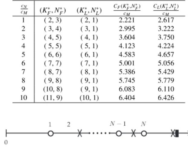
We compute numerically optimal (K^∗_F,N_F^∗) and (K_L^∗,N^∗_L) when c_N = c_K,G(t) = 1−e^−tandH(t) =(λt)². Tables 2 and 3 give (K_F^∗,N^∗_F), CF(K_F^∗,N_F^∗)/cM, (K_L^∗,N_L^∗) andC_L(K^∗_L,N_L^∗)/c_M forc_N/c_M = 1,2, . . .10 whenλ = 0.1 andλ =1, respectively. We can see from these tables that CF(K_F^∗,N_F^∗)/c_M <CL(K^∗_L,N_L^∗)/c_M.

5. Overtime Policies

5.1 Replacement at First Failure Over CycleN

Suppose that the unit is replaced at the first failure over working cycleN (N =0,1,2, . . .) (see Fig. 5). Recall that F(t)=1−e^−H(t) and the probability that the unit with aget fails in (u,u+du] foru >tis f(u)du/F(t). Thus, the mean

Table 2 Optimal (K^∗_F,N^∗_F),CF(K_F^∗,N^∗_F)/cM, (K^∗_L,N^∗_L) andCL(K^∗_L,N_L^∗)/

cMwhenG(t)=1−e^−t,H(t)=(λt)²,cN=cKandλ=0.1.

c_N

c_M (K_F^∗,N_F^∗) (K^∗_L,N^∗_L) ^CF(K

∗ F,N^∗_F) c_M

C_L(K^∗_L,N_L^∗) c_M

1 ( 3, 11) ( 0, 9) 0.208 0.210

2 ( 4, 15) ( 1, 13) 0.291 0.292

3 ( 5, 19) ( 2, 16) 0.354 0.355

4 ( 6, 22) ( 3, 18) 0.407 0.408

5 ( 7, 25) ( 4, 20) 0.454 0.455

6 ( 8, 27) ( 5, 22) 0.496 0.497

7 ( 9, 30) ( 6, 24) 0.535 0.536

8 (10, 32) ( 7, 25) 0.572 0.572

9 (11, 34) ( 8, 26) 0.606 0.607

10 (12, 36) ( 9, 28) 0.638 0.639

Table 3 Optimal (K^∗_F,N^∗_F),C_F(K_F^∗,N^∗_F)/cM, (K^∗_L,N^∗_L) andC_L(K^∗_L,N_L^∗)/

c_MwhenG(t)=1−e^−t,H(t)=(λt)²,c_N=c_Kandλ=1.0.

c_N

c_M (K_F^∗,N^∗

F) (K^∗_L,N^∗

L) ^CF(K

∗ F,N^∗_F) cM

CL(K^∗_L,N_L^∗) cM

1 ( 2, 3) ( 2, 1) 2.221 2.617

2 ( 3, 4) ( 3, 1) 2.995 3.222

3 ( 4, 5) ( 4, 1) 3.604 3.750

4 ( 5, 5) ( 5, 1) 4.123 4.224

5 ( 6, 6) ( 6, 1) 4.583 4.657

6 ( 7, 7) ( 7, 1) 5.001 5.056

7 ( 8, 7) ( 8, 1) 5.386 5.429

8 ( 9, 8) ( 9, 1) 5.745 5.779

9 (10, 8) ( 9, 1) 6.083 6.110

10 (11, 9) (10, 1) 6.404 6.426

Fig. 5 Replacement at first failure over cycleN.

time to replacement is Z ∞

0

1 F(t)

"Z ∞

t

udF(u)

# dG^(N)(t)

= N

θ +Z ∞

0

"Z ∞

t

e^−H(u)+H(t)du

# dG^(N)(t)

=µ+Z ∞ 0

h1−G^(N)(t)i"Z ∞ t

e^−H(u)+H(t)du

#

h(t)dt, (26) and the expected number of failures until replacement is

Z ∞

0

1 F(t)

"Z ∞

t

H(u)dF(u)

# dG^(N)(t)

=1+Z ∞ 0

[1−G^(N)(t)]h(t) dt. (27) Thus, the expected cost rate is

CO(N)= c_ON+c_Mn 1+R∞

0

h1−G^(N)(t)i h(t)dto µ+R∞

0

1−G^(N)(t)hR∞

t e^−H(u)+H(t)dui h(t)dt

. (28) wherecON =replacement cost at first failure over cycleN.

We find optimal N_O^∗ to minimizeCO(N) whenG(t) =

528

1−e^−θt. Forming the inequalityC_O(N+1)−C_O(N)≥0, QO1(N)

( µ+Z ∞

0

h1−G^(N)(t)i"Z ∞ t

e^−H(u)+H(t)du

# h(t)dt

)

− Z ∞

0

[1−G^(N)(t)]h(t)dt−1≥ cON

c_M, (29) where

QO1(N)≡

R∞

0 (θt)^Ne^−θth(t) dt R∞

0 (θt)^Ne^−θth(t)hR∞

t e^−H(u)+H(t)dui dt

, which increases strictly withN toh(∞) from Appendix E.

Thus, because the left-hand side of (29) increases strictly withN to∞, there exists a finite and unique minimumN_O^∗ (0 ≤ N_O^∗ < ∞) which satisfies (29), and the resulting cost rate is

cMQO1(N_O^∗−1)<CO(N_O^∗)≤cMQO1(N_O^∗). (30) 5.2 Replacement at First Cycle Over FailureK

Suppose that the unit is replaced at the first working cycle over failureK(K=0,1,2, . . .) (see Fig. 6). The mean time to replacement is

∞

X

j=0

Z ∞

0

(Z t

0

"Z ∞

t

ydG(y−u)

#

dG^(j)(u) )

dPK(t)

=Z ∞ 0

PK(t)dt +

∞

X

j=0

Z ∞

0

(Z t

0

"Z ∞

t

G(y−u)dy

#

dG^(j)(u) )

dP_K(t)

=1 θ

∞

X

j=0

Z ∞

0

G^(j)(t)dPK(t), (31)

and the expected number of failures until replacement is

∞

X

j=0

Z ∞

0

(Z t

0

"Z ∞

t

H(y)dG(y−u)

#

dG^(j)(u) )

dPK(t)

=

∞

X

j=0

Z ∞

0

(Z t

0

"Z ∞

t

G(y)h(u+y)dy

# dG^(j)(u)

) dP_K(t).

(32) Therefore, the expected cost rate is

CO(K)= c_OK+c_MP∞

j=0

R∞ 0 {Rt

0[R∞

0 G(y)h(u+y)dy]dG^(j)(u)}dP_K(t) (1/θ)P∞

j=0

R∞

0 G^(j)(t)dP_K(t) . (33)

Fig. 6 Replacement at first cycle over failureK.

wherec_OK =replacement cost at first cycle over failureK.

In particular, whenG(t)=1−e^−θt, CO(K)=

c_OK+c_M{R∞

0 e^−θth(t)dt+R∞

0 P_K(t)[R∞

0 θe^−θuh(t+u)du]dt}

1/θ+R∞

0 P_K(t)dt .

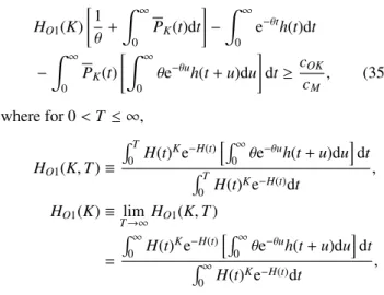
(34) We find optimalK_O^∗ to minimizeCO(K) in (34). Form- ing the inequalityCO(K+1)−CO(K)≥0,

HO1(K)

"

1

θ+Z ∞

0

P_K(t)dt

#

− Z ∞

0

e^−θth(t)dt

− Z ∞

0

P_K(t)

"Z ∞

0

θe^−θuh(t+u)du

#

dt≥c_OK cM

, (35)

where for 0<T ≤ ∞, HO1(K,T)≡

RT

0 H(t)^Ke^−H(t)hR∞

0 θe^−θuh(t+u)dui dt RT

0 H(t)^Ke^−H(t)dt

, HO1(K)≡ lim

T→∞HO1(K,T)

= R∞

0 H(t)^Ke^−H(t)hR∞

0 θe^−θuh(t+u)dui dt R∞

0 H(t)^Ke^−H(t)dt , which increases strictly withK toR∞

0 θe^−θth(T +t)dtfrom Appendix F. Thus, because the left-hand side of (35) in- creases strictly withKto∞, there exists a finite and unique minimum K_O^∗ (0 ≤ K_O^∗ < ∞) which satisfies (35), and the resulting cost rate is

c_MH_O1(K_O^∗ −1)<C_O(K^∗_O)≤c_MH_O1(K_O^∗). (36) We discuss numerically optimalN_O^∗, K_O^∗ whencON = c_OK, G(t) = 1−e^−t and H(t) = (λt)². Tables 4 and 5 give optimal N_O^∗,CO(N^∗), K_O^∗,CO(K_O^∗) when λ = 0.1 and λ = 1, respectively. We can see from these tables that CO(N_O^∗)<CO(K^∗_O) forcON/cM ≤5 andCO(N_O^∗) ≥CO(K_O^∗) forcON/c_M≥6 in Table 4,CO(N_O^∗)<CO(K_O^∗) forcON/c_M≤ 3 andCO(N_O^∗) ≥CO(K_O^∗) forcON/cM ≥4 in Table 5. This means thatcON/c_M has a threshold level and ifcON/c_M is smaller than this level, i.e., replacement cost is relatively

Table 4 OptimalN^∗_O,C_O(N_O^∗)/c_M,K_O^∗,C_O(K^∗_O)/c_M, whenG(t)=1− e^−t,H(t)=(λt)²andc_ON=c_OK,λ=0.1.

c_ON/cM N^∗_O ^CO(N

∗ O)

c_M K_O^{∗ CO(K}

∗ O) c_M

1 6 0.216 1 0.223

2 11 0.294 2 0.300

3 14 0.357 3 0.361

4 17 0.410 4 0.412

5 20 0.457 5 0.458

6 22 0.500 6 0.500

7 24 0.539 7 0.539

8 26 0.576 8 0.575

9 28 0.610 9 0.608

10 30 0.643 10 0.641

Table 5 OptimalN_O^∗,CO(N^∗_O)/cM,K^∗_O,CO(K_O^∗)/cM, whenG(t)=1− e^−t,H(t)=(λt)²andc_ON=c_OK,λ=1.

c_ON/cM N_O^{∗ CO(N}

∗ O)

c_M K_O^{∗ CO(K}

∗ O) c_M

1 1 2.702 1 3.060

2 1 3.377 1 3.590

3 1 4.052 1 4.121

4 1 4.728 2 4.576

5 2 5.231 2 5.005

6 2 5.667 3 5.381

7 2 6.103 4 5.743

8 2 6.539 4 6.084

9 3 6.885 5 6.401

10 3 7.198 6 6.707

smaller against minimal repair costc_M, replacement at first failure over cycleNis better than replacement at first cycle over failureK.

6. Conclusions

We have discussed theoretically and numerically the opti- mal policies of replacements with cycleNand failureK. In general, it would be more difficult to derive theoretically op- timal policies for replacements with discrete variables than those with continuous ones. This paper has given several mathematical techniques of solving optimization problems with discrete variables and these would be useful for main- tenances of actual models in practical fields. For example, we can propose the following replacement policies from the results of this paper:

1. IfcN is smaller thancK and cycle N can be counted more easily than failureK, then cycleNis better than failureK.

2. Ifc_K is smaller than c_N and failureK can be counted more easily than cycleN, then failureKis better than cycleN.

3. IfcK is smaller thancN and cycle N can be counted more easily than failureK, then replacement overtime with cycleNis better than failureK.

4. IfcN is smaller than cK and failureK can be counted more easily than cycleN, then replacement overtime with failureKis better than cycleN.

5. If both costs ofc_Nandc_K are almost the same and cy- cleNand failureKcan be counted easily, we compute the expected costsC(N^∗) andC(K^∗), and the expected costsC(N_F^∗,K_F^∗) andC(N_L^∗,K^∗_L) numerically, and de- cide the optimal replacement policy.

The replacement policies proposed in this paper would be applied to the cumulative damage models and data backup models of computer systems by making some suit- able modifications[19],[20].

Acknowledgments

This work is supported by JSPS KAKENHI Grant Number 18K01713, National Natural Science Foundation of China (NO. 71801126), Natural Science Foundation of Jiangsu

Province (NO. BK20180412) and Fundamental Research Funds for the Central Universities (NO. NR2018003).

References

[1] R.E. Barlow and F. Proschan, Mathematical Theory of Reliability, John Wiley & Sons, New York, 1965.

[2] S. Osaki, Stochastic Models in Reliability and Maintenance, Springer Verlag, Berlin, 2002.

[3] T. Nakagawa, Maintenance Theory of Reliability, Springer Verlag, London, 2005.

[4] T. Nakagawa, Advanced Reliability Models and Maintenance Poli- cies, Springer Verlag, London, 2008.

[5] T. Nakagawa, Random Maintenance Policies, Springer Verlag, Lon- don, 2014.

[6] W. Stadje, “Renewal analysis of a replacement process,” Oper. Res.

Lett., vol.31, no.1, pp.1–6, 2013.

[7] M. Chen, S. Mizutani, and T. Nakagawa, “Random and age replace- ment policies,” Int. J. Rel. Qual. Saf. Eng., vol.17, no.1, pp.27–39, 2010.

[8] M. Chen, S. Nakamura, and T. Nakagawa, “Replacement and pre- ventive maintenance models with random working times,” IEICE Trans. Fundamentals, vol.E93-A, no.2, pp.500–507, 2010.

[9] C. Chang, “Optimum preventive maintenance policies for systems subject to random working times, replacement, and minimal repair,”

Comput. Ind. Eng., vol.67, pp.185–194, 2014.

[10] M. Hamidi, F. Szidarovszky, and M. Szidarovszky, “New one cycle criteria for optimizing preventive replacement policies,” Reliab. Eng.

Syst. Safe., vol.154, pp.42–48, 2016.

[11] S. Sheu, T. Liu, Z. Zhang, and H. Tsai, “The general age mainte- nance policies with random working times,” Reliab. Eng. Syst. Safe., vol.169, pp.503–514, 2018.

[12] S. Sheu, H. Tsai, U. Sheu, and G. Zhang, “Optimal replacement policies for a system based on a one-cycle criterion,” Reliab. Eng.

Syst. Safe., vol.191, 106527, 2019.

[13] M. Berrade, P. Scarf, and C. Cavalcante, “A study of postponed re- placement in a delay time model,” Reliab. Eng. Syst. Safe., vol.168, pp.70–79, 2017.

[14] T. Nakagawa, X. Zhao, and W. Yun, “Optimal age replacement and inspection policies with random failure and replacement times,” Int.

J. Rel. Qual. Saf. Eng., vol.18, no.5, pp.405–416, 2011.

[15] X. Zhao and T. Nakagawa, “Optimization problems of replacement first or last in reliability theory,” Eur. J. Oper. Res., vol.223, no.1, pp.141–149, 2012.

[16] X. Zhao and T. Nakagawa, “Optimal periodic and random inspection with first, last, and overtime policies,” Int. J. Syst. Sci., vol.46, no.9, pp.1648–1660, 2013. DOI: 10.1080/00207721.2013.827263 [17] X. Zhao, S. Mizutani, and T. Nakagawa, “Which is better for re-

placement policies with continuous or discrete scheduled times?,”

Eur. J. Oper. Res., vol.242, no.2, pp.477–486, 2015.

[18] T. Nakagawa and X. Zhao, Maintenance Overtime Policies in Reli- ability Theory, Springer Verlag, London, 2015.

[19] X. Zhao and T. Nakagawa, Advanced Maintenance Policies for Shock and Damage Models, Springer Verlag, London, 2018.

[20] X. Zhao and T. Nakagawa, “Over-time and over-level replacement policies with random working cycles,” Ann. Oper. Res., vol.244, no.1, pp.103–116, 2016.

Appendix A:

ForN=0,1,2, . . .,K=1,2, . . . and 0<T <∞, Q2(N,K;T)≡

RT

0 (θt)^Ne^−θtPK(t)h(t)dt RT

0 (θt)^Ne^−θtPK(t)dt ,

530

which increases strictly withNfromQ2(0,K;T) toh(T) and increases strictly withKfromQ2(N,1;T) to

Q2(N;∞;T)= RT

0 (θt)^Ne^−θth(t)dt RT

0 (θt)^Ne^−θtdt .

Proof. Note that Q2(∞;K;T)= lim

N→∞

RT

0 (θt)^Ne^−θtPK(t)h(t)dt RT

0 (θt)^Ne^−θtP_K(t)dt =h(T), Q2(N;∞;T)=

RT

0 (θt)^Ne^−θth(t)dt RT

0 (θt)^Ne^−θtdt .

Denoting L1(T)≡

Z T

0

(θt)^N+1e^−θtPK(t)h(t)dt Z T

0

(θt)^Ne^−θtPK(t)dt

− Z T

0

(θt)^Ne^−θtPK(t)h(t)dt Z T

0

(θt)^N+1e^−θtPK(t)dt, we haveL1(0)=0 and

L⁰₁(T)=(θT)^Ne^−θTPK(t)

× Z T

0

(θt)^Ne^−θtPK(t)(θT −θt)[h(T)−h(t)]dt>0, which follows that Q2(N,K;T) increases strictly with N from Q2(0,K;T) toh(T) for anyK andT. Similarly, de- noting

L2(T)≡

K

X

j=0

Z T

0

(θt)^Ne^−θtpj(t)h(t)dt

K−1

X

j=0

Z T

0

(θt)^Ne^−θtpj(t)dt

−

K−1

X

j=0

Z T

0

(θt)^Ne^−θtpj(t)h(t)dt

K

X

j=0

Z T

0

(θt)^Ne^−θtpj(t)dt,

we haveL2(0)=0 and L⁰₂(T)=(θT)^Ne^−θT

K−1

X

j=0

Z T

0

(θt)^Ne^−θt[h(T)−h(t)]

×e^{−H(T)−H(t)}

K!j! [H(T)H(t)]^j[H(T)^K−j−H(t)^K−j]dt>0, which follows that Q2(N,K;T) increases strictly with K fromQ₂(N,1;T) toQ₂(N;∞;T) for anyN andT. There- fore, because T is arbitrary, Q2(N,K) ≡ Q2(N,K;∞) increases strictly with N from Q2(0,K) to h(∞) and increases strictly with K from Q2(N,1) to Q1(N) = θR∞

0 [(θt)^N/N!]e^−θth(t)dt, and becauseKis arbitrary,Q1(N) increases strictly withNtoh(∞).

Appendix B:

ForN=1,2, . . .,K=0,1,2, . . . and 0<T <∞,

H2(N,K;T)= PN−1

j=0

RT

0 [(θt)^j/j!]e^−θtp_K(t)h(t)dt PN−1

j=0

RT

0 [(θt)^j/j!]e^−θtpK(t)dt ,

which increases strictly withNfromH2(1,K;T) to H2(∞,K;T)=

RT

0 p_K(t)h(t)dt RT

0 p_K(t)dt ,

and increases strictly withNfromH2(N,0;T) toh(T).

Proof. Note that H2(∞,K;T)=

RT

0 p_K(t)h(t)dt RT

0 p_K(t)dt ,

H2(N,∞;T)≡ lim

K→∞

PN−1 j=0

RT

0 [(θt)^j/j!]e^−θtpK(t)h(t)dt PN−1

j=0

RT

0 [(θt)^j/j!]e^−θtpK(t)dt

=h(T).

Denoting L₃(T)≡

Z T

0

[(θt)^N/N!]e^−θtp_K(t)h(t)dt

N−1

X

j=0

Z T

0

[(θt)^j/j!]e^−θtp_K(t)dt

− Z T

0

[(θt)^N/N!]e^−θtpK(t)dt

N−1

X

j=0

Z T

0

[(θt)^j/j!]e^−θtpK(t)h(t)dt,

we haveL3(0)=0 and L⁰₃(T)=

N−1

X

j=0

Z T

0

e^−θ(T+t)pK(T)pK(t)[h(T)−h(t)]

×(θT)^N(θt)^j−(θT)^j(θt)^N N!j! dt>0,

which follows that H₂(N,K;T) increases strictly with N fromH2(1,K;T) toH2(∞,K;T) for anyKandT. Similarly, denoting

L4(T)≡

N−1

X

j=0

Z T

0

(θt)^j

j! e^−θtp_K+1(t)h(t)dt

N−1

X

j=0

Z T

0

(θt)^j

j! e^−θtp_K(t)dt

−

N−1

X

j=0

Z T

0

(θt)^j

j! e^−θtpK(t)h(t)dt

N−1

X

j=0

Z T

0

(θt)^j

j! e^−θtpK+1(t)dt, we haveL4(0)=0 and

L⁰₄(T)=

N−1

X

j=0

(θT)^j j! e^−θT

N−1

X

j=0

Z T

0

(θt)^j

j! e^−θt[H(T)H(t)]^K K!(K+1)!

×e^{−H(T)−H(t)}[H(T)−H(t)][h(T)−(t)]dt>0, which follows that H2(N,K;T) increases strictly with K from H2(N,0;T) toh(T) for any NandT. Therefore, be- cause T is arbitrary, H2(N,K) ≡ H2(N,K;∞) increases