Outline ( ) / 10

1

章 序論

東京大学

2014

Outline

1 1.1 統計学の概要 2 1.2 データ 3 _{1.3 データの収集} 4 1.4 確率の計算 5 1.5 仮説検定

Outline

1 1.1 統計学の概要 2 1.2 データ 3 _{1.3 データの収集} 4 1.4 確率の計算 5 1.5 仮説検定 (東京大学) 1章 序論 2014 2 / 10

Outline

1 1.1 統計学の概要 2 1.2 データ 3 1.3 データの収集 4 1.4 確率の計算 5 1.5 仮説検定

Outline

1 1.1 統計学の概要 2 1.2 データ 3 1.3 データの収集 4 1.4 確率の計算 5 1.5 仮説検定 (東京大学) 1章 序論 2014 2 / 10

Outline

1 1.1 統計学の概要 2 1.2 データ 3 1.3 データの収集 4 1.4 確率の計算 5 1.5 仮説検定

統計学とは

一言で言えば・・・ データを収集し、それを分析する学問 データから何を分析するのか？ 母集団 (population): データの抽出元、データを生成する構造自体 統計学の目的： 母集団そのものの性質を調べること 例: 日本の内閣支持率を考える。「母集団」は？ 母集団＝有権者全員。 データ（「標本」）＝有権者の一部に対する聞き取り調査の結果。 (東京大学) 1章 序論 2014 3 / 10

記述統計と推測統計

記述統計 : データを分かりやすく記述する。 推測統計: データから母集団の特性を推測する。 Remark 全数調査が可能であれば、データは母集団と一致し、その特性を直接知 ることができる。しかし、多くの場合、全数調査は時間とコストの両面 から困難であり、推測統計が必要となる。 例: テレビの視聴率

データ

例：身長のデータ (X1, X2, X3, X4, X5) = (172.9, 180.3, 142.1, 120.2, 172.3) 変数の種類： 連続変数 : 連続的な値をとりうる変数：身長、体重・・・ 離散変数: 離散的な値だけを取りうる変数：ある試合で勝ち負けを記録したデータ （勝ったら1、負けたら0）、内閣支持率調査のデータ（支持すると答えた ら1、支持しないと答えたら0） (東京大学) 1章 序論 2014 5 / 10

データの種類： 時系列データ (time-series data): 時間の経過とともに観測されるデー タ。例えば、1974∼ 2011年の東京都の県内総生産の記録。 横断面データ (cross-section data): ある1時点において複数の対象を記録したデータ。例えば、1975年だけ の47都道府県の県内総生産。 パネルデータ (panel data): 横断面データが複数年にまたがって利用できる場合。例えば、 1974∼ 2011年の47都道府県の県内総生産の記録。

データの収集

データは、できるだけ偏り(バイアス)なく、母集団を代表するデータを 取り出す必要がある。 バイアスのあるデータの分析からは、バイアスのある結果が出てし まう。 例えば、大学生の意識調査をする時に、友人にだけ聞取り調査をす ると、母集団である大学生を代表していない可能性がある。なぜか？ 「類を友を呼ぶ」 (東京大学) 1章 序論 2014 7 / 10

バイアスの発生を回避する方法：無作為抽出(random sampling)=母集 団を構成するどの個体もデータとして選ばれる確率が同じになる抽出法。 現実には誤ったデータ抽出が頻繁に行われている。 例えば、1936年の米国大統領選において、『リテラシー・ダイジェス ト』誌が勝利者を予想するため、電話や自動車の保有者などから選 ばれた約237万人に聞取り調査を行った結果、共和党候補ランドン 氏が圧倒的な優勢となった。しかし、実際の選挙では民主党候補 ルーズベルト氏の勝利となった。なぜ調査結果は誤ったか？ Remark 社会調査では、無作為抽出のほかにも、1.面接員の質問の仕方、2.質問 の設定の仕方、3.回答者が嘘をつく可能性等にも、注意を払う必要があ る。（教科書1.3.2節参照）

1.4確率の計算

確率の計算

直観は頼りになるか？ 例：HIV検査の偽陽性問題 HIV検査において、感染者については100%の確率で陽性反応が出る が、非感染者でも検査に反応する抗体を持っている可能性があり、1%の 確率で陽性反応を示すとする。全人口の0.1%だけが感染者であると仮定 した場合、陽性の検査結果が出た時、その人がHIVに感染している確率 はどのくらいだろうか？ 9% (東京大学) 1章 序論 2014 9 / 10

確率の計算

直観は頼りになるか？ 例：HIV検査の偽陽性問題 HIV検査において、感染者については100%の確率で陽性反応が出る が、非感染者でも検査に反応する抗体を持っている可能性があり、1%の 確率で陽性反応を示すとする。全人口の0.1%だけが感染者であると仮定 した場合、陽性の検査結果が出た時、その人がHIVに感染している確率 はどのくらいだろうか？ 9%

仮説検定

(hypothesis testing)

仮説がデータと整合的かどうかを検証する方法。 「帰無仮説」 (null hypothesis): 検証したい仮説。 「対立仮説」 (alternative hypothesis): 帰無仮説が誤っていたとき の受け皿としての仮説。 仮説検定は、これらの仮説を設定した上で、どちらの仮説がデータ と整合的であるかを判断する。 例：太郎君が、「気になる女性がある社内の別の男性と恋愛中であるかど うか」をその二人が有給休暇を取っているタイミングの「データ」をも とに「仮説検定」したい。 帰無仮説：「二人の間に恋愛関係がない」 対立仮説：「二人の間に恋愛関係がある」 二人の有給休暇を調べた結果、タイミングが完全に一致していた。 太郎君は、これを偶然と考えるのには無理があると判断し、「二人の 間に恋愛関係がある」、つまり「対立仮説」が正しいと判断した。 (東京大学) 1章 序論 2014 10 / 10

2

章 データの記述

東京大学

Outline

1 図表の作成

2 標本特性値

Outline

1 図表の作成

図表の作成

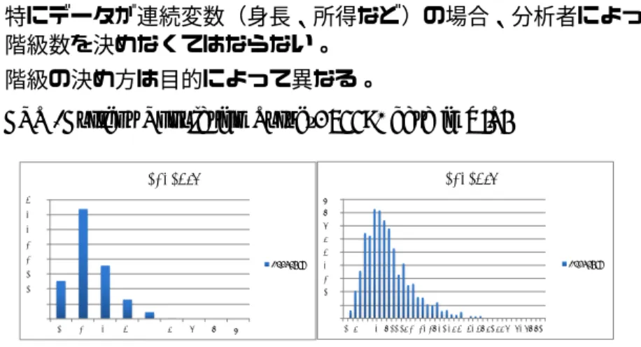
例：ある工場における従業員の欠勤日数のデータ（一年間） (X1, . . . , X50) = 6, 4, 4, 6, 0, 6, 11, 5, 10, 8, 4, 8, 4, 7, 7, 3, 2, 3, 6, 2 4, 3, 6, 1, 3, 2, 4, 6, 6, 6, 6, 8, 3, 3, 6, 2, 3, 2, 4, 0 8, 3, 6, 0, 1, 6, 5, 13, 11, 6 度数分布表(frequency table) ヒストグラム (histogram) (東京大学) 2章 データの記述 2014 3 / 19

度数分布表：データの大きさによっていくつかの組（階級）に分けて、 度数 (各組に入る観測値の数）をまとめた表 階級値：観測値が属する各組の中心値 相対度数：総度数に対する各度数の割合 累積相対度数：相対度数を下から順に加えてその累積値を求めたもの ヒストグラム：各階級の度数を長方形によりグラフ表示したもの。 0   2   4   6   8   10   12   14   0   1   2   3   4   5   6   7   8   9   10   11   12   13  

number  of  days  absent  

特にデータが連続変数（身長、所得など）の場合、分析者によって 階級数を決めなくてはならない。

階級の決め方は目的によって異なる。

例：CPS (Current Population Survey, 2008) data in U.S.

0   500   1000   1500   2000   2500   3000   3500   4000   10   20   30   40   50   60   70   80   90   frequency   frequency   0   100   200   300   400   500   600   700   800   900   2   6   10  14  18  22  26  30  34  38  42  46  50  54  58  62  66  70  74  78  82   frequency   frequency  

Figure : Hourly earnings in the United States of Working Graduates, Ages 28-34

in 2008 Dollars

代表的分布の形状 釣鐘状の分布：左右対称な釣鐘状の分布。(適切に設計された試験の 成績、身長、株価の変化率など) 右に歪んだ分布：右裾が長く、左裾が短い分布。(所得、資産、結婚 年齢、体重など) 左に歪んだ分布：左裾が長く、右裾が短い分布。(簡単な試験の成 績、人間の寿命など)

中心を表す標本特性値

1. 平均 (mean) 以下、データを(x1, x2, . . . , xn)とする。平均は以下で定義される。 平均 ¯ x = 1 n n ∑ i =1 xi 平均には、外れ値の影響を受けやすいという欠点がある。 例えば、{1, 2, 3, 4, 5}というデータが与えられた場合、平均は (1 + 2 + 3 + 4 + 5)/5 = [ ]。 ここで、何らかの原因で5の代わりに90という外れ値がデータに含 まれているとする。このとき、新しいデータ{1, 2, 3, 4, 90}の平均は (1 + 2 + 3 + 4 + 90)/5 = [ ]となり、外れ値の影響を大きく受け ることになる。 (東京大学) 2章 データの記述 2014 7 / 19

2. 中央値 (median) まず、データを小さい順（昇順）に並べ直す（x₍₁₎≤ x₍₂₎ ≤ · · · ≤ x_(n))。 中央値（median）は以下で定義される。 中央値 nが奇数なら：x_(n+1)/2 nが偶数なら： x(n/2)+x(n/2+1) 2 中央値は、外れ値の影響を受けない。 {1, 2, 3, 4, 5}というデータの中央値は[ ]。 {1, 2, 3, 4, 90}の中央値は[ ]。

3. 最頻値 (mode) 最頻値（mode）は、 最頻値 「最大の頻度を持つ測定値」 として定義される。 度数分布表が与えられている時には（階級幅が同じという条件の下 で）最大度数を与える階級の階級値を最頻値とする。 最頻値も外れ値の影響を受けない。 (東京大学) 2章 データの記述 2014 9 / 19

中心を表す

3

つの特性値の使い方

平均、中央値、最頻値の3つの値を相互比較することによって有用な情 報が得られる。 分布が釣鐘状なら、[ = = ] 分布が右に歪んでいるなら、[ < < ] 分布が左に歪んでいるなら、[ < < ] 従って、特性値を相互比較することによって、分布の形状をおおまかに 推測できる。

ばらつきを表す標本特性値

例：試験の成績 グループA：40点、42点、58点、60点 グループB：20点、35点、45点、100点 両グループとも、平均は50点。 グループAは点数のばらつきが小さく、Bはばらつきが大きい。 Aは平均を中心に狭い範囲でばらつき、Bは平均を中心に広範囲に 散らばっている。 −→ ばらつきの指標を作るために、平均からの乖離を考える。 ID番号iの人の点数xi の平均x¯からの乖離xi− ¯x を偏差 (deviation)と呼ぶ。 しかし、全て偏差を足し合わせるだけでは、全体のばらつきを測る ことはできないことに注意する。(∑n_{i =1}(xi − ¯x) = 0.) −→ 「偏差の二乗を足し合わせたもので、全体のばらつきを測る」とい う考え方による指標。 (東京大学) 2章 データの記述 2014 11 / 19

標本分散 (sample variance) s_x2 = 1 n− 1 n ∑ i =1 (xi − ¯x)2 除数をサンプルサイズnではなく、n− 1としている理由は後ほど 説明。 標本分散は偏差の二乗をもとに求めた値であるため、桁数がデータ の桁数から変わってしまう。 データのばらつきの直観をつかむために、標本分散の平方根をとっ たものを標本標準偏差 (sample standard deviation)と呼ぶ。

標本標準偏差 (sample standard deviation) sx = v u u t 1 n− 1 n ∑ i =1 (xi − ¯x)2 先ほどの点数の例では、グループAは、 s_x2 = [ ] sx = [ ] グループBは、 s_x2 = [ ] sx = [ ] (東京大学) 2章 データの記述 2014 13 / 19

データの線形変換

例：入試の得点調整 世界史：平均70点、標準偏差15点 日本史：平均50点、標準偏差10点 このままでは世界史の平均が高いため、日本史で受験した学生に不 利になる可能性あり。 そこで、日本史の得点の平均と標準偏差を世界史のそれに合わせる という得点調整を考える。 具体的には、日本史の点数がxiのとき、yi = a + bxi と線形変換し、 得点調整後の日本史の得点yi の平均(¯y )が70点、標準偏差(sy)が 15点となるようにa,bを選ぶ。

ここで、次の関係が成り立つことに注意する。 ¯ y = a + b¯x , s_y2= b2s_x2, sy =|b|sx 今、¯x = 50、sx = 10なので、¯y = 70, sy = 15となるためには、連立方 程式 70 = a + 50b, 15 = 10b を解いて、a = [ ], b = [ ]とすればよい。 (東京大学) 2章 データの記述 2014 15 / 19

線形変換のイメージ

yi = a + xi, a > 0の場合：分布の[ ]は変わらないが、 [ ]だけ[ ]にシフトした分布になる。 yi = bxi, b > 1の場合：分布の[ ]は変わらないが、 [ ]が[ ]なった分布になる。 yi = bxi, 0 < b < 1の場合：分布の[ ]は変わらない が、[ ]が[ ]なった分布になる。

yi = bxi, b =−1の場合：xの分布の[ ]した分布 となる。 yi = bxi, −1 < b < 0の場合：xの分布を[ ]し、 [ ]が[ ]なった分布になる。 yi = bxi, b <−1の場合：xの分布を[ ]し、 [ ]が[ ]なった分布になる。 (東京大学) 2章 データの記述 2014 17 / 19

範囲と割合の関係

経験的に（厳密にはデータが「正規分布」と呼ばれる分布に従う場合）、 範囲と割合の間には次のような関係が成り立つことが知られている。 範囲 割合 ¯ x± sx 約68% ¯ x± 2sx 約95% ¯ x± 3sx 約99∼ 100% 例：偏差値 iさんの偏差値= 50 + 10 ( xi − ¯x sx ) 偏差値40∼60の間に全体の約68%、偏差値30∼70の間に全体の約 95%、偏差値20∼80の間に全体の約99∼100%が入る。

3

章 相関

東京大学

2014

Outline

1 図表の作成

Outline

1 図表の作成

2 標本共分散と標本相関係数

散布図

散布図 (scatter plot): 2変数からなるデータ (x , y )を平面上の点として プロットしたもの。 例：モネ(Monet)の絵画オークションのデータ -­‐5   -­‐4   -­‐3   -­‐2   -­‐1   0   1   2   3   4   0   1   2   3   4   5   6   7   8   9   10   Log  Pr ic e Log  Area

Log  Price  vs.  Log  Area  for  Monet  Pain3ngs  

散布図から分かる3つの関係： 正の相関がある場合：xが高いとyも高い場合（教育と賃金の関係 など） 負の相関がある場合：xが高いとyが低い場合（喫煙量と寿命の関 係、駅からの距離と地価の関係など） 相関がない場合：xとyの動きに関連性が見られない場合 例：為替レートの変化率 (東京大学) 3章 相関 2014 4 / 9

標本共分散

標本共分散 (sample covariance)は、2変数の共変動を表す指標であり、 標本共分散がプラスなら正の相関、マイナスなら負の相関、0なら無相 関、0に近いなら相関が弱いとされる。 標本共分散 (sample covariance) sxy = 1 n− 1 n ∑ i =1 (xi − ¯x)(yi − ¯y) 例：太郎君、次郎君、三郎君の身長xと体重yが次のとおりだったと する。 (180cm, 80kg), (170cm, 70kg), (160cm, 60kg) この時、x = [¯ ]、y = [¯ ]なので、

標本共分散の欠点：スケール（尺度）が変わると、その値も変わってし まう。 たとえば、cm表示からm表示に変更すると、標本共分散は[ ] 倍されてしまう。 −→ この問題を解決する指標が標本相関係数 (sample correlation coefficient) (東京大学) 3章 相関 2014 6 / 9

標本相関係数 (sample correlation coefficient) rxy = sxy sxsy 標本相関係数は、標本共分散と符号は同じ。 標本相関係数は、スケール変更に依存しない。 標本相関係数は、-1から1の間の値を取る。 標本相関係数が1または-1となるのは、変数xとyに完全な線形関 係(y = a + bx )が成立しているとき。 例：先ほどの3兄弟の身長と体重の標本相関係数は rxy = [ ]

標本相関係数の注意点

1．相関と因果関係は異なる概念である。 相関は両変数の動きに関連性があるかを示す概念であるのに対し、 因果関係は原因と結果という関係を意味する概念である。 xとyに相関があっても、それはxからyへの因果なのか、yからx への因果なのか、あるいは両方の因果が混ざっているのかは分から ない。 (両方の因果が混ざっている場合の例)：選挙資金と選挙結果の間には正の 相関があるが、「選挙資金が当選を決める重要な要因である」とはいえ ない。 (相関があっても因果関係を全く意味しない例「見せかけの相関」)：溺死 者数とアイスクリーム消費量の間には正の相関があるが、それは「夏の 暑さ」によって生まれたものであり、両者に因果関係はない。 (東京大学) 3章 相関 2014 8 / 9

2. 標本相関係数でとらえることができるのは線形関係だけである。 例: 電力需要と気温の関係はU字型となる。そのため、相関係数では変 数間の相互関係を上手くとらえることはできない。

4

章 確率

東京大学

2014

Outline

1 4.1 標本空間

Outline

1 4.1 標本空間

2 4.2 確率

推測統計は確率論に基づいて行われる。また、確率論の基礎は集合論で ある。ここでは、まず集合論の基本概念を概観する。 Definition 結果が偶然に支配される実験を試行 (trial)という。 試行により生じる実現可能な全ての結果を集めたものを標本空間 (sample space)といい、Ωで表す。 標本空間の個々の異なった結果を標本点 (sample point)といい、ω で表す。 標本空間の部分集合を事象 (event)という。 Example 1: コイン投げの試行の場合、 標本空間は表と裏,すなわち Ω ={H, T }. Example 2: 「一組の夫婦が三人の子供を産む」という試行の場合、一つ の標本点は例えばBGB、すなわち「男の子、次に女の子、最後に男の子」 となる。標本空間は、

Example 1, continued: コイン投げにおいて、可能な全ての事象(all possible events)は

[H, T , Ω, ϕ] .

である。ここで、ϕは空事象 (null event)という。

二つの事象AとBが与えられた場合、次のように集合演算を定義する。 Definition 和事象 (Union): AとBの少なくとも一方が起こる事象 A∪ B = {x : x ∈ A or x ∈ B}. 積事象 (Intersection): AとBが同時に起こる事象 A∩ B = {x : x ∈ A and x ∈ B}. 余事象 (Complement): Aの余事象は、「Aが起こらない事象」 ¯ A ={x : x /∈ A}.

Example 3: トランプからカードを取り出す試行において、カードのマー ク (club(C), diamonds(D), hearts(H), or spades(S))に注目する。標本空 間は Ω ={ }, であり、事象には、例えば A ={C, H}, B ={C, D, S}. が含まれる。このとき、 A∪ B = { }, A ∩ B = { }, ¯A = { }. (東京大学) 4章 確率 2014 6 / 22

「確率」を 以下のように定義する。 Definition ある事象Aが起こる確率とは、観察回数nと事象Aが起こった回数n(A) との相対度数n(A)/nの極限値である。 Pr (A) = lim n→∞ n(A) n . 例えば、サイコロの各目が出る確率は、サイコロを何度も投げた後、そ の目が観測される相対度数の極限値（相対度数が近づいていく値）とし て定義される。歪みのないサイコロであれば、各目の確率は1/6となる。

The following is more rigorous definition of “probability”, which is optional.

Definition

Definition(optional): A collection of subsets of Ω is called a sigma algebra (or Borel field), denoted by B, if it satisfied the following three properties:

a. ϕ∈ B, where ϕ is the empty set. b.If A∈ B, then ¯A ∈ B.

c.If A1, A2, . . . ,∈ B, then ∪∞i =1Ai ∈ B.

Definition

Definition(optional): Given a sample space Ω and associated sigma algebra B, a probability function is a function P with domain B that satisfies

1. P(A)≥ 0 for all A ∈ B. 2. P(Ω) = 1.

3. If A1, A2, . . . ,∈ B are mutually exclusive (i.e., do not overlap), then

P(∪∞_{i =1}Ai) = ∑_∞

i =1P(Ai).

Example 2, continued: 一組の夫婦が3人の子供を産む例において、す べての出産において男の子が生まれる確率と女の子が生まれる確率がそ れぞれ50%であるとする。この時、 「男の子→女の子→男の子」とな る「確率」は？ Pr (BGB) = [ ]. 夫婦が次のような事象を望んでいるとする。 E =少なくとも2人は女の子 この時、 Pr (E ) = [ ]. (1/2)

次のような事象を考える。 F = 少なくとも１人は女の子 G = 女の子は2人未満 H = 全ての子の性別が同じ K = 男の子が2人未満 I = 女の子なし Pr (I∪ K) = [ ]. (5/8) Pr (G∪ H) = [ ]. (5/8) Pr (F ) = [ ]. (7/8) 便利な公式： Pr (A∪ B) = Pr(A) + Pr(B) − Pr(A ∩ B). Pr (A) = 1− Pr(¯A). (東京大学) 4章 確率 2014 10 / 22

事象AとBが互いに共通点を持たない(片方の事象が起こったら、もう 片方は絶対に起こらないような)時、二つの事象は互いに排反 (disjoint or mutually exclusive) であるという。 例えば、事象I と事象K は排反である。 便利な公式： 事象AとBが排反なら、 Pr (A∪ B) = Pr(A) + Pr(B)

条件付確率

(Conditional Probability)

Example 2, continued：3人の子供を産む例において、事象G (女の子が 二人未満)が起こったとする。この時、事象H (全ての子の性別が同じ) となる確率は？ この確率を「事象Gが起こったという条件のもとで、事象Hが起こる条 件付確率 (conditional probability) 」といい、次のように定義される。 Definition 事象Gが起こったという条件のもとで、事象Hが起こる条件付確率 (conditional probability) Pr (H|G) = Pr (H∩ G) Pr (G ) . (東京大学) 4章 確率 2014 12 / 22

(a)男の子が生まれる確率が50%の時、Pr (H|G)は？

Pr (H|G) = [ ] (1/4)

(b) 男の子が生まれる確率が52%の時、Pr (H|G)は？

（例）お隣さんの飼っている犬が2匹の子犬を産みました。お隣さんは 「少なくとも1匹はオスでしたよ」と教えてくれました。この時、残りの 犬もオスである確率は何%でしょうか？（オスが産まれる確率は50%で あるとする。） （答）2匹ともオスである場合を事象A、少なくとも1匹がオスである場 合を事象Bとする。 Pr (A|B) = Pr (A∩ B) Pr (B) = Pr (MM) Pr (MM, MF , FM) = 1/4 3/4 = 1 3. (東京大学) 4章 確率 2014 14 / 22

条件付確率の定義から、次の公式が成り立つ。 Theorem

Pr (G ∩ H) = Pr(G)Pr(H|G)

Example 4: Suppose that 3 defective light bulbs inadvertently got mixed with 6 good ones. If 2 bulbs are chosen at random for a ceiling lamp, what is the probability that they both are good?

Answer: Let us denote

G1 = first bulb is good

G2 = second bulb is good

Thus,

Pr (both good) = Pr (G1 ∩ G2)

独立

(Independence)

Definition 事象AはBと独立 (statistically independent)であるとは、 Pr (A|B) = Pr(A), が成立することである。（事象Aが起こる確率は事象Bが起こった後にA が起こる確率と同じ。）すなわち、事象AがBと独立である時、Bという 情報はAの確率に何の影響も与えない。 条件付確率の定義から、より一般に次のことが成り立つ。 Definition Pr (A∩ B) = Pr(A)Pr(B) が成り立つなら、AとBは独立 (statistically independent)である。 (東京大学) 4章 確率 2014 16 / 22

ベイズの定理

(Bayes’ Theorem)

(例) あなたの上司は温厚な人で99.9%の人とは上手に付き合っており、 残り0.1%の人とだけ仲が悪いとする。上司は仲の良い人には1%の確率 で返事が遅れ、仲の悪い人には100%の確率で返事が遅れるとします。 上司からの返事が遅いとき、その理由は上司があなたを嫌っているから である確率はどのくらいだろうか？ Theorem ベイズの定理 (Bayes’ Theorem)：互いに排反な事象A1, A2を原因事象と し、Bを結果事象とする。このとき、結果Bが原因A1によって生じたも のである確率は、 Pr (A1|B) = Pr (B|A1)P(A1) Pr (B) = Pr (B|A1)P(A1) Pr (B|A1)Pr (A1) + Pr (B|A2)Pr (A2) となる。

3-23 The table below classifies the 115.5 million civilians in the 1985 U.S. labor force by age and employment status (Stat. Abst. of U.S.,1987, p.378):

Age

Y (young, under 25) O (older, 25 and over) Totals

E (employed) 20.4 86.8 107.2

U (unemployed) 3.2 5.1 8.3

Totals 23.6 91.9 115.5 million

a. What is Pr (U), the probability that a worker drawn at random will be unemployed? That is, find the unemployment rate.

b. What is Pr (U|Y )?

c. Is unemployment independent of age?

3-18: Suppose that 4 defective light bulbs inadvertently have been mixed up with 6 good ones.

a. If 2 bulbs are chosen at random, what is the chance that they both are good?

b. If the first 2 are good, what is the chance that the next 3 are good? c. If we started all over again and chose 5 bulbs, what is the chance they all would be good?

3-35: Suppose that A and B are independent events, with Pr (A) = .6 and Pr (B) = .2. What is a. Pr (A|B)? b. Pr (A∩ B)? c. Pr (A∪ B)? (東京大学) 4章 確率 2014 20 / 22

3-36 Repeat Problem 3-35 if A and B are mutually exclusive instead of independent.

3-45: True or False? If false, correct it:

a. When two events are independent, the occurrence of one event will not change the probability of the second event.

b. Two events are mutually exclusive if they have no outcomes in common. c. Two events are mutually exclusive if Pr (A∩ B) = Pr(A)Pr(B).

d. If a fair coin has been fairly tossed 5 times and has come up tails each time, on the sixth toss the conditional probability of tails will be 1/64.

5

章 確率変数と確率分布

東京大学

離散確率変数

(Discrete Random Variables)

Example 2, continued: 一組の夫婦が3人の子供を産みたいと考えてお り、「女の子の数」に興味を持っているとする。この場合、 X =女の子の数 とすると、X は確率変数 (random variable)と呼ばれる。Xの取り得る 値は [ ]である。 例えば、女の子の産まれる確率が48%であるとする。 確率変数Xの取り得る各値xに対する確率を計算するためには、元の標 本空間に戻る必要がある。 (例) Pr (X = 1) = [ ] (.39) (東京大学) 5章 確率変数と確率分布 2014 2 / 42

同様にして、Xの取り得る各値xに対する確率は以下のように計算で きる。 p(0) ≡ Pr(X = 0) = [ ] (.14) p(1) ≡ Pr(X = 1) = [ ] (.39) p(2) ≡ Pr(X = 2) = [ ] (.36) p(3) ≡ Pr(X = 3) = [ ] (.11) 以上の確率をまとめて 確率分布 (probability distribution)と呼ぶ。 確率分布を用いることで、次のような問いに答えることもできる：「女の 子が2人未満の確率は？」 Pr (X < 2) = p(0) + p(1) = [ ] (.53)

期待値

(expectation)

、分散

(variance)

、標準偏差

(

standard deviation)

Xの確率分布が分かると、事前にXの期待値、分散、標準偏差を求める ことができる。 Definition 離散確率変数Xの取り得る値を{x1, . . . , xm}とする。 Mean µ = E [X ] = m ∑ i =1 xip(xi) Variance σ2 = V (X ) = n ∑ i =1 (xi − µ)2p(xi) Standard Deviation σ = v u u t∑n i =1 (xi − µ)2_p(x i) (東京大学) 5章 確率変数と確率分布 2014 4 / 42

分散 σ2_{の計算のためには、次の便利な公式がある。} 便利な公式 σ2= m ∑ i =1 x_i2p(xi)− µ2

Example 2, continued: 前と同じ例において、Xの期待値、分散、標準 偏差はどうなるだろうか？(We suppose that the probability of a boy is 52%.) X = 3人の子供の中で女の子の数. Mean µ = [ ] (1.44) Variance σ2 = [ ] (.75) Standard Deviation σ = [ ] (.87) (東京大学) 5章 確率変数と確率分布 2014 6 / 42

二項分布

(Binomial Distribution)

離散確率変数には様々な種類のものがあるが、最も重要なものは二項(確 率)変数(binomial variable)と呼ばれる。 二項確率変数の古典的な例： S = n回の独立なコイン投げにおいて表が出る回数. 一般に、ある試行において、特定の事象Aが起これば成功、それ以外で あれば失敗とする。この時、成功回数Sは二項(確率)変数 (binomial variable)と呼ばれる。

Examples： S = 三人の子供のうちの女の子の数 S = 選択式（ex. 5択）の質問に当てずっぽうに答えた場合の正解数 S = 選挙において無作為に選ばれた投票者中の共和党支持者の数 S = 一日の工場生産において無作為に選ばれた製品の中の不良品の数 (東京大学) 5章 確率変数と確率分布 2014 8 / 42

n回の独立試行における「成功」数をSとする。各試行の成功確率をπ とする時、n回のうちs回成功する確率は次のように表される。 二項分布の確率関数 p(s) = ( n s ) πs(1− π)n−s (1) where ( n s ) ≡ n! s!(n− s)!, and n! ≡ n(n − 1)(n − 2) · · · 1 例えば、前の子供の性別の例で、女の子の数が1人となる確率は、 n = [ ], π = [ ], and s = [ ]を(1)に代入して p(1) = [ ] (.39)

Derivation of the binomial formula (1):

Let’s consider a tossing coin n = 5 times. We suppose the coin is somewhat biased, coming up H with probability π = .60, and T with probability 1− π = .40. Here, let’s calculate the probability that the number of H, S = 3. The

generalization is straightforward.

One of the many ways we could get S = 3 is

HHH TT ,

whose probability is

(.60)(.60)(.60)(.40)(.40) = (.60)3(.40)2.

But there are many other ways we could get exactly 3 heads in 5 tosses. For example, we might get the sequence (THTHH), which has a probability

(.40)(.60)(.40)(.60)(.60) = (.60)3(.40)2,

which is the same probability as before. In fact, all sequences in the event S = 3 will have this same probability.

Finally, how many ways are there to get exactly 3 heads? The answer is the number of of different ways that three H’s and and two T’s can be arranged. The number of arrangements of five distinct objects is

5· 4 · 3 · 2 · 1 = 5!,

but we over-counted (3· 2 · 1)(2 · 1) times. So the number of ways is ( 5 3 ) = 5! 3!2! = 10. Hence we have p(3) = ( 5 3 ) (.60)3(.40)2 = 10(.035) = .35

Example: How reliable is a small poll?

Suppose that a sample of 5 voters is to be randomly drawn from the U.S. population, when 60% vote Republican.

(a) The number of Republican voters in this sample of 5 can vary anywhere from 0 to 5. Tabulate its probability distribution. (b) Calculate the mean and standard deviation of the number of Republican voters in this sample.

(c) What is the probability of exactly 3 Republican voters in the sample? (35%)

(d) Calculate the probability that the sample will have a majority of Republican voters (that is, at least 3) and thus will correctly reflect the population majority. (68%)

連続確率変数

(continuous random variables)

確率変数Xの取りうる値が連続的な場合、Xは連続確率変数である という。 X が連続確率変数の場合、取りうる値は無数に存在するため、特定 の点に有限の「確率」を付与すると全ての確率の和が無限になって しまう。そこで、確率は（点ではなく）幅に対して定義し、密度関 数f (x )を次のように定義する。 連続確率変数の場合の確率と密度関数 Pr (a≤ X ≤ b) = ∫ b a f (x )dx . 確率の和は1なので、次の事実が成り立つ。 Pr (−∞ ≤ X ≤ ∞) = ∫ _∞ f (x )dx = 1.

正規分布

(Normal Distribution)

正規分布は、次のような理由で統計において最も重要な分布である。

(i) Empirically, many random variables have bell-shaped probability densities which are very close to the normal distribution.

(ii) Errors made in measuring physical and economic phenomena often are normally distributed.

(iii) Many other probability distributions (such as the binomial) often can be approximated by the normal curve.

(iv) There is a famous theorem (Central Limit Theorem): The distribution of sum of ANY random variables approaches the normal distribution as the number of the observations increases (under some conditions). This fact will be very useful in statistical inference.

正規分布 (Normal Distribution)

以下の密度関数を持つ確率変数を正規確率変数 (Normal random variable、その分布を正規分布 (Normal distribution)という。

f (x ) = √ 1 2πσ2e −(x−µ)2 2σ2 正規確率変数Xの期待値はµ、分散はσ2となる。 Xが正規分布に従うことを X ∼ N(µ, σ2) と表す。

標準正規分布

(Standard Normal Distribution)

正規確率変数のうち、特に期待値µ = 0、分散σ2= 1であるものを、特 に標準正規確率変数 (Standard normal random variable)といい、その 分布を標準正規分布 (Standard normal distribution)という。

標準正規分布 (Standard normal distribution)

以下の密度関数を持つ確率変数を正規確率変数、その分布を正規分布と いう。 f (x ) = √1 2πe −x 2 2 (東京大学) 5章 確率変数と確率分布 2014 16 / 42

「標準正規確率変数Zがある値以上(あるいは以下）になる確率」に興味 があるとする。

この確率は、統計家によって既に計算されており、標準正規分布表にま とめられている。

この表を使って以下のような確率も計算することができる。

Example: If Z has a standard normal distribution, find: a. Pr (Z > 1.64)

b. Pr (Z <−1.64) c. Pr (1.0 < Z < 1.5) d. Pr (−1 < Z < 2) e. Pr (−2 < Z < 2)

一般の正規分布

(General Normal Distribution)

In general, a normal distribution may have any mean µ, and any standard deviation σ. For example, when the population of American men have their height X arrayed into a frequency distribution, it looks a normal distribution with mean µ = 69 inches, and standard deviation σ = 3 inches.

Question: How could we calculate the proportion of men above 74 inches, for example?

The important fact we use is

Z = X−µ_σ follows the standard normal distribution when X is normally distributed with mean µ and standard deviation σ.

Since we have the table of tail probabilities of the standard normal distribution (the standard normal table), we can calculate

Pr (X > 74) = Pr (X − µ σ >

74− µ

σ )

= Pr (Z > 1.67)≈ 5% (we use the stander normal table here) Sometimes, we say that

4-20: If X is normally distributed around a mean of 16 with a standard deviation of 5, find a. Pr (X > 20) b. Pr (X < 10) c. Pr (20 < X < 25) d. Pr (12 < X < 24) (東京大学) 5章 確率変数と確率分布 2014 20 / 42

確率変数の関数の期待値

Since means play a key role in statistics, they have been calculated by all sorts of people, who sometimes use different names for the same concept. For example, geographers use the term “mean annual rainfall,” teachers use the term “average grade,” and gamblers and economists use the term “expected profit.”

We often use the the following notation E called “expected value”, and define in general

Definition

E [g (X )] =∑ x

g (x )p(x )

As an example, one possible form of the function g (x ) is: g (X ) = (X− µ)2. Then we have E [(X − µ)2] =∑ x (x− µ)2p(x ), which equals to the variance of X . Hence we can write

Variance σ2 = E [(X − µ)2]. In the new E notation, we also can rewrite (2) as

σ2= E (X2)− µ2

4-10: In families with 6 children, let X = the number of boys. For simplicity, assume that births are independent and boys and girls are equally likely.

a. Graph the probability distribution of X .

b. Calculate the mean and standard deviation, and show them on the graph.

c. Of all families with 6 children, what proportion have: i. Exactly an even split between the sexes (3-3)? ii. Nearly an even split (3-3 or 4-2 or 2-4)? iii. 3 or more boys?

4-22: The time required to complete a college achievement test was found to be normally distributed, with a mean of 110 minutes and a standard deviation of 20 minutes.

a. What proportion of the students will finish in 2 hours (120 minutes)? b. When should the test be terminated to allow just enough time for 90% of the students to complete the test?

4-25: In her new job of selling computers, Dawn Elliot faces uncertain prospects next year. She guesses that her taxable income X might be anywhere from 20 to 50 thousand dollars according to her schedule of personal probabilities p(x ) given below. The corresponding tax is given in the final column.

Income x ($000) Probability p(x ) Tax t(x ) ($000)

20 0.1 4

30 0.3 6

40 0.4 9

50 0.2 13

a. Calculate her expected income. b. Calculate her expected tax.

c. Calculate her expected disposable income (after tax) in two ways: i. Calculate first the table of disposable incomes, and then take their expected value.

複数の確率変数：同時確率分布

(Joint Distributions)

There are many cases we want to consider two random variables at the same time. In the planning of three children, let us denote two random variables:

X = number of girls Y = number of runs

where a run is an unbroken string of children of the same sex. For example, Y = 1 for the outcome BBB, while Y = 2 for the outcome BBG .

Suppose that we are interested in the probability that a family would have 1 girl and 2 runs, Pr (X = 1 and Y = 2)? (We assume that the probability of a boy is 52%.)

Pr (X = 1 and Y = 2) = [ ] which we simply denote by p(1, 2).

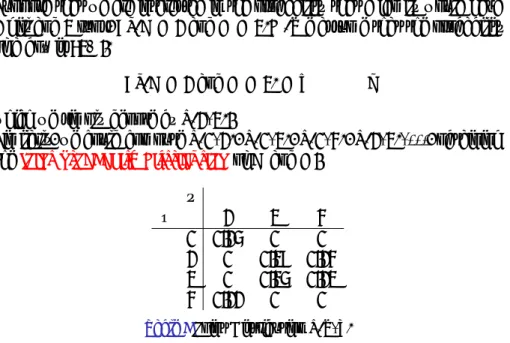
Similarly, we could compute p(0, 1), p(0, 2), p(0, 3), p(1, 2), . . ., obtaining thejoint probability distribution of X and Y .

y x 1 2 3 0 0.14 0 0 1 0 0.26 0.13 2 0 0.24 0.12 3 0.11 0 0

周辺確率分布

(Marginal Distributions)

Suppose that we are interested only in X , yet have to work with the joint distribution of X and Y . For any given x , we define the marginal distribution of x : Xの周辺分布 pX(x ) = ∑ y p(x , y ). For example, pX(2) = p(2, 1) + p(2, 2) + p(2, 3) = ∑ y p(2, y ) Of course, the distribution of Y can be calculated in a similar way:

Yの周辺分布 pY(y ) = ∑ x p(x , y ). (東京大学) 5章 確率変数と確率分布 2014 28 / 42

独立

(Independence)

Definition

X and Y are independent if

p(x , y ) = p(x )p(y ) for all x and y .

For the distribution in Table 1, are X and Y independent? Answer: [ ]

複数の確率変数の関数の期待値

Suppose we are interested in the expected value of some function of X and Y , g (x , y ). We define it E [g (X , Y )] =∑ x ∑ y g (x , y )p(x , y ),

which is similar to the earlier formula E [g (X )] =∑

x

g (x )p(x )

in the one variable case.

共分散と相関係数

One of the most interesting questions in the face of two variables are how they vary together or how they are related. In this section we will develop how they can be measured. We define thecovariancefirst, which is given by

σXY = Covariance of X and Y ≡ E[(X − µX)(Y − µY)] where µX = E [X ] and µY = E [Y ].

The calculation of the covariance can often be simplified by using an alternative formula:

σXY > 0 indicates the positive relation between X and Y (when one is large, the other tends to be [ ].)

σXY < 0 indicates the negative relation between X and Y (when one is large, the other tends to be [ ].)

If X and Y are independent, then they are uncorrelated (σXY = 0).

Since the covariance depends on the units in which X and Y are

measured, 1 it is not a good measure of the strength of the relation of the two variable. We define the correlation ρ which is completely independent of the scale in which either X and Y is measured.

Correlation, ρ≡ σXY σXσY

Now suppose that X and Y have a perfect positive linear relation. For example, suppose they always take on the same values, so that X = Y . Then it is easy to show that ρ takes on [ ].

Similarly, if there is a perfect negative linear relation, then ρ would be

[ ].

In fact, ρ is always bounded:

−1 ≤ ρ ≤ 1.

5-15: Does education make you happy?

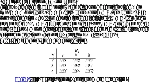
Americans were asked in 1971 to rank themselves on a “happiness index” as follows: H = 0 (not happy), H = 1 (fairly happy), or H = 2 (very happy). The amount of education was also measured for each individual: X = 1 (elementary school completed), X = 2 (high school completed), or X = 3 (college completed, or more). Thus X = number of schools completed. Then the relative frequencies of various combinations were roughly as follows (Gallup, 1971):

a: Calculate the covariance and correlation.

h

x 0 1 2

1 0.02 0.08 0.05

2 0.02 0.28 0.25

3 0.01 0.13 0.16

b: Answer True or False; if False, correct it.

i. As X increases, the average level of H increases. This positive relation is reflected in a positive correlation ρ.

ii. Yet the relation is just a tendency (H fluctuate around its average level), so that ρ is less than 1.

iii. This shows that those who receive high education tend to be happier than the poor, that is, education tends to make people happier.

Linear combination of Two Random Variables

E [X + Y ] = E [X ] + E [Y ]

E [aX + bY ] = aE [X ] + bE [Y ] for any constants a and b.

Proof: E [aX + bY ] = ∑ x ∑ y (ax + by )p(x , y ) = a∑ x x (∑ y p(x , y )) + b∑ y y (∑ x p(x , y )) = a∑ x xp(x ) + b∑ y yp(y ) = aE (X ) + bE (Y ) (東京大学) 5章 確率変数と確率分布 2014 38 / 42

Variance

Var (X + Y ) = Var (X ) + Var (Y ) + 2Cov (X , Y )

Var (aX + bY ) = a2Var (X ) + b2Var (Y ) + 2ab Cov (X , Y ) for any constants a and b.

Proof: Var (aX + bY ) = ∑ x ∑ y

{(ax + by) − (aµx+ bµy)}2p(x , y )

= ∑ x ∑ y {a(x − µx) + b(y− µy)}2p(x , y ) = ∑ x ∑ y {a2_{(x− µ} x)2+ b2(y− µy)2+ 2ab(x− µx)(y− µy)}p(x, y) = a2∑ x ∑ y (x− µx)2p(x , y ) + b2 ∑ x ∑ y (y− µy)2p(x , y ) +2ab∑ x ∑ y (x− µx)(y− µy)p(x , y ) = a2Var (X ) + b2Var (Y ) + 2ab Cov (X , Y )

Example: Investors often prefer to have a portfolio whose expected profit is as high as possible and variance is as low as possible. How can we construct such a “nice” portfolio?

Suppose there are two assets X and Y with E [X ] = 5, E [Y ] = 5,

Var (X ) = 1, Var (Y ) = 1. What are the expected profit and the variance of the portfolio Z = 1₂X +1₂Y in the following three cases?

a. When Cov (X , Y ) = 0.3. b. When Cov (X , Y ) =−0.3. c. When X and Y are independent.

If X and Y are independent,

Var (X + Y ) = Var (X ) + Var (Y )

Var (aX + bY ) = a2Var (X ) + b2Var (Y ) for any constants a and b.