Earthquake Risk and Housing Prices in Japan: Evidence Beforeand After Massive Earthquakes

JOINT RESEARCH CENTER FOR PANEL STUDIES

DISCUSSION PAPER SERIES

DP2009-001 August, 2009

Earthquake Risk and Housing Prices in Japan:

Evidence Beforeand After Massive Earthquakes

Michio Naoi* Miki Seko** Kazuto Sumita***

Abstract

The hedonic pricing approach is used to examine whether homeowners and/or renters alter their subjective assessments of earthquake risks after massive earthquakes. Using nation-wide household panel data coupled with earthquake hazard information and records of observed earthquakes, we find that there are some modifications of individuals’ assessments of earthquake risk in both cases. We have carefully taken into consideration the bias stemming from the use of objective risk variables as a proxy for individual risk assessments. Our results suggest that the price discount from locating within a

quake-prone area is significantly larger soon after earthquake events than beforehand. We argue that the most likely interpretation for this result is that households tend to

underestimate earthquake risk if there has not been a recent occurrence.

*Michio Naoi

Faculty of Economics, Keio University

** Miki Seko

Faculty of Economics, Keio University

*** Kazuto Sumita

Department of Economics, Kanazawa Seiryo University

Joint Research Center for Panel Studies

Keio University

1

Earthquake Risk and Housing Prices in Japan: Evidence Before

and After Massive Earthquakes

*

First draft: May28, 2008

First revision: June 29, 2009

Michio Naoi

a

, Miki Seko

b†

, Kazuto Sumita

c

a. Faculty of Economics, Keio University, Mita Toho Bldg. 3

rd

Floor, 3-1-7 Mita,

Minato-ku, Tokyo, 108-0073, Japan

b. Faculty of Economics, Keio University, 2-15-45 Mita, Minato-ku, Tokyo, 108-8345,

Japan

c. Department of Economics, Kanazawa Seiryo University, Ushi 10-1, Gosho-machi,

Kanazawa-shi, Ishikawa, 920-8620, Japan

* _{We are grateful to the National Research Institute for Earth Science and Disaster Prevention (NIED) for}

generously providing us with the data on earthquake hazard information. We also thank Richard Arnott, Eric Hanushek, Dwight Jaffee, Charles Leung, Colin McKenzie, Tsunao Okumura, John Quigley, Tim Riddiough, James Shilling, Jay Weiser, Jiro Yoshida, two anonymous referees and participants at the Macro, Real Estate and Public Policy Workshop, the 12th AsRES Annual Conference and the International Conference on Economic Analysis and Policy Evaluation Using Panel Data for their helpful comments. Financial support from the Japan Economic Research Foundation is gratefully acknowledged. The first author (Michio Naoi) acknowledges a Grant-in-Aid (#19730183) for Young Scientists from the Ministry of Education, Culture, Sports, Science and Technology. The second and third authors (Miki Seko and Kazuto Sumita) acknowledge a Grant-in-Aid (#19530157) for Scientific Research (C) from the Ministry of Education Culture, Sports, Science and Technology.

†

2

Abstract

The hedonic pricing approach is used to examine whether homeowners and/or renters

alter their subjective assessments of earthquake risks after massive earthquakes. Using

nation-wide household panel data coupled with earthquake hazard information and

records of observed earthquakes, we find that there are some modifications of individuals’ assessments of earthquake risk in both cases. We have carefully taken into consideration

the bias stemming from the use of objective risk variables as a proxy for individual risk

assessments. Our results suggest that the price discount from locating within a

quake-prone area is significantly larger soon after earthquake events than beforehand. We

argue that the most likely interpretation for this result is that households tend to

underestimate earthquake risk if there has not been a recent occurrence.

JEL classification: R20, C23.

3

1. Introduction

Japan is one of the world’s most earthquake-prone countries since it lies at the nexus of four tectonic plates. A recent survey reports that Japan averaged 1.14 earthquake events equal to or

greater than a magnitude of 5.5 on the Richter scale a year between 1980 and 2000, which

according to the United Nations Development Program is fourth highest among 50 countries

surveyed (UNDP, 2004). It is assumed that these massive earthquakes increase awareness of

earthquake risk among individuals, largely due to extensive media coverage of the event and the

resulting quake damages. Indeed, sales of earthquake insurance policies increased by 75% in

Hyogo Prefecture in 1995, immediately after the Great Hanshin-Awaji (Kobe) Earthquake, and

by nearly 25% in Miyagi Prefecture after the 2003 Miyagi Earthquake, while the corresponding

nation-wide increases were only 29% and 5% respectively.

If existing government anti-seismic policies are efficient in the sense that earthquake risks

are properly assessed and individuals are well-informed about these risks, major tremors should

not alter individuals’ perception toward risk. Therefore, modifications of individuals’ perceptions after an earthquake indicates that there is room for improvement in the current

anti-seismic policies concerning risk assessment and its dissemination among the public.

In this paper, we use a hedonic pricing approach to estimate individuals’ valuation of

earthquake risk. The nation-wide household longitudinal data coupled with earthquake hazard

information and the observed earthquake record allows us to investigate whether individuals,

i.e., homeowners and renters, alter their subjective assessments of earthquake risks after an

earthquake. Using a difference-in-differences (DID) approach with longitudinal data, we find

that there are some post-quake modifications of individuals’ assessments of earthquake risk. Our

4

risk, both housing rents and owner-occupied home values are significantly and negatively

correlated with regional earthquake risk in post-quake periods. The most plausible interpretation

for these results is that both renters and homeowners are initially unaware of, or at least

underestimate, earthquake risk. We also conduct several robustness checks on our main

empirical findings, and compare the homeowner’s implicit price estimates with capitalized insurance premiums.

The paper is organized as follows. Section 2 briefly reviews the previous studies of

earthquake risk in the housing market. Section 3 presents a simple theoretical framework.

Section 4 introduces the data used and explains estimation methods and variables. Section 5

presents empirical results and interpretation. Section 6 summarizes the paper and presents some

conclusions.

2. Previous Studies

Since an earthquake is an exogenous risk factor that is tied to a specific location, its risk should

be capitalized into local housing and land prices. Estimating individuals’ valuation of

earthquake risk is crucial for evaluating the benefits of earthquake damage mitigation policies.

There have been relatively few studies on the effect of earthquake risk on housing and land

prices despite the obvious relevance to effective disaster prevention policies. Brookshire, Thayer,

Tschirhart, and Schulze (1985) examine the effects of the disclosure of a risk hazard map in

California on sales prices of single-family houses. It is found that the earthquake hazard indices

do have a significantly negative impact on prices after they are disclosed. Nakagawa, Saito, and

Yamaga (2009) empirically investigate the effect of earthquake risk on land prices using the

5

Metropolitan Government. Their results suggest that higher earthquake risk is clearly related to

lower land prices in each area. Nakagawa, Saito, and Yamaga (2007) examine the impact of

earthquake risk on housing rents in the Tokyo Metropolitan Area with special reference to the

new Building Standard Law enacted in 1981, using the same earthquake risk index used by

Nakagawa et al. (2009). They find that housing rents are substantially lower in the areas of

higher earthquake risk. Also, they find that the rent of houses built prior to 1981 is discounted

more substantially in risky areas than for houses built after 1981.

Beron, Murdoch, Thayer, and Vijverberg (1997) conduct hedonic analysis of residential

housing prices in the San Francisco Bay area using the expected loss from earthquakes as an

additional explanatory variable, and compare the estimated hedonic functions before and after

the 1989 Loma Prieta Earthquake.1 The result indicates that the hazard indices have a

significantly negative impact on housing prices in both time periods; however, its impact is

greater in the pre-earthquake period, implying that earthquake risk was overestimated before the

Loma Prieta Earthquake occurred. Significantly, they focus only on the area actually hit by the

earthquake, and their results are obtained by simply comparing before and after the earthquake

without any relevant control group. Thus, their results may reflect some other factors that render

earthquake risk less important over time such as improvement in quake-resistant construction

technology.

Compared with previous studies, our contributions are as follows. First, while previous

studies mainly focus on small areas that are subject to a specific earthquake event, we use

1

There are also several studies about the relationship between flood hazards and housing prices in the US. Among others, Bin and Polasky (2004) and Hallstrom and Smith (2005) investigate the effect of specific hurricane events – Floyd and Andrew – on individuals’ perception of flood risks. Shilling, Benjamin and Sirmans (1987), MacDonald, Murdoch, and White (1987), MacDonald, White, Taube, and Huth (1990) and Bin, Kruse, and Landry (2008) have also evaluated the effect of flood hazard on housing values.

6

nation-wide longitudinal data that covers areas with near-miss incidents of massive earthquakes,

i.e. whose neighboring city/towns were recently hit by a massive earthquake, as well as those

without any such experiences. Since housing prices are influenced by various factors varying

over time, a simple before-after comparison within a small area might yield misleading

conclusions. Second, we use longitudinal data rather than (repeated) cross-section data in our

analysis. By observing the same households repeatedly, we can control for individual

heterogeneity that influences housing price changes over time. Further, we carefully examine

the bias stemming from the use of objective risk variables as a proxy for subjective assessments,

utilizing the panel data instrumental variables estimator. Third, we examine whether

homeowners and renters alter their subjective assessments of earthquake risks after massive

earthquakes. To the best of our knowledge, there has been no prior attempt to analyze the effects

of earthquake risk on property values before and after a major earthquake event for both

homeowners and renters.

3. Theoretical Considerations

Hedonic pricing model with uncertain hazardous events

In this section, we present a simple hedonic pricing model to illustrate household responses to

the prospect of hazardous events and the effect of additional information on perceptions toward

risk. A similar model is also presented in MacDonald et al. (1987) and Kask and Maani (1992).

The basic intuition of the model is that household’s valuation of the different bundles of housing and location characteristics leads to differential housing costs. Thus, the observed discount on

property in a hazardous area reflects households’ risk assessment and willingness to pay to avoid such risk. In our context, given that a massive earthquake can have a potentially

7

catastrophic impact on each household, and that the risk is generally fairly differentiated across

regions, it is quite natural to expect that households will incorporate earthquake risk into their

decision on choice of location. Rational households are willing to pay an additional amount for

houses located in an area where the probability of hazard is less. Conversely, rational

households may choose to locate within quake-prone areas only if they are compensated for

their risk in terms of discounted housing prices that can offset the potential loss and damage

from a major seismic event.

Let us assume that there are two states, 0 and 1, corresponding to a “no earthquake” and “earthquake” situation. Let



be the probability of earthquake occurrence (i.e., the probability assigned to state 1). Hedonic pricing method suggests that housing cost can be described as a

function of both housing/structural characteristics and location-specific characteristics (such as

environmental factors and neighborhood quality). In our context, differentiated risk of

earthquake will be a particularly important factor influencing the market cost of housing. Hence,

the hedonic price function can be written as:

 

h

,



,

p

p



(1)

where

p

is the observed housing cost (e.g., rental price or sales price of a particular housing

unit), and h is a vector of housing and location-specific characteristics that are not related to

earthquake risk.

A household maximizes its expected utility by choosing a bundle of housing characteristics

and level of earthquake risk.2 Let

u ,

 

h

x

be the utility function, where

x

is an amount of numeraire goods consumption, with

u

_h



_

0

and

u

_x



0

. Let

y

0 and

y

1 be the state-contingent income where we assume

y

0



y

1 with

L



y

0



y

1 being the monetary

2 _{The preferred level of earthquake risk can be achieved by choosing a particular location of residence or}

8

loss from the earthquake. Then the household’s budget constraint suggests that the numeraire

goods consumption under two states can be written as 0 0

 

,



h

p

y

x





and

 

,



1 1

h

p

y

x





, respectively. The household’s expected utility to be maximized can be represented as:3

 



,

,





1





,

 

,



.

max

1 0 ,

EU



U

h

y

p

h





U

h

y

p

h



h











(2)

The first-order conditions give us the equilibrium conditions required for optimal levels of

the j th housing/location-specific characteristics and earthquake risk.







1



0

,

1

0 1 0 1





















x x h h j h

U

U

U

U

h

p

p

j j j









(3)



1



0

0

,

1 0 1

















x x

U

U

U

U

p

p







 (4)

where

U

1 and

U

0, respectively, represent the utility when the earthquake occurs and when it

does not, and subscripts denote partial derivatives. Equation (3) indicates that the implicit price

for any housing/location characteristics reflects the expected (dis-) amenity value. Equation (4)

indicates that the implicit price for the probability of earthquake occurrence reflects a utility

difference across states,

U

1



U

0. Since the right-hand-side of both equations (3) and (4) are divided by the expected marginal utility of numeraire goods consumption,



U1_x



1





U_x0, these implicit price estimates provide a convenient way to evaluate the marginal willingness to

pay (MWP) in this simplified situation.

3 _{Alternatively, Kask and Maani (1992) assume that households will optimally choose the level of}

self-protection expenditure that reduces the risk of damage from an earthquake event. The different specification of the model, however, does not change our main theoretical result.

9

The effect of earthquake insurance

In the simplified situation above, the housing market will completely respond to the potential

risk of earthquakes, and any differentiated earthquake risk will be capitalized into differentiated

housing costs across regions. However, in reality, households can hedge against earthquake risk

through the purchase of insurance policies. In order to examine the effect of the insurance

market, we assume, in a simplified way, that earthquake insurance offers a contract with a

known amount of insurance claims paid when state 1 occurs

 

m

for the annual insurance premium

r

 



that can vary across regions depending on earthquake probability. In this case, equation (4) can be rewritten as:



1



0

,

1 0 1  

_

_

r

U

U

U

U

p

x x











(5)

where

r

_ is the marginal increase in an insurance premium.

Equation (5) has at least two important implications for our benchmark result. First, in

equation (5), the implicit price for the probability of earthquake occurrence

 

p

_ is no longer equal to the household’s MWP as in equation (4). This is because regional earthquake risks are partly reflected in the differentiated premiums in the insurance market. Since we expect that the

true MWP (i.e., the first term on the right-hand-side) should be negative, and that the insurance

premium is generally higher in risky regions (i.e.,

r

_



0

), the implicit price for earthquake probability would overestimate the true MWP. In all, the estimates for household’s MWP should

be given by

p

_



r

_. Secondly, if the claim paid by the insurer is perceived to be equal to the loss from the earthquake



m



L



, then income, and thus utility level, in the two states will be equal (i.e., U1 U0). Under these special conditions, equation (5) suggests that the implicit price estimate should be equal to the negative of the premium increment,

p

_





r

_. Several studies utilize this relationship to test the expected utility theory (MacDonald et al., 1987; Bin

10

and Polasky, 2004; Bin et al., 2008). If, instead, the claim paid by the insurer is perceived to be

less than the losses caused by the earthquake, then the household’s MWP would be negative



1 0



U

U



, and the expected relationship would be

p

_





r

_. In this case,

p

_



r

_ is the uninsured component of earthquake risk, i.e., the household’s MWP under partial coverage

insurance.

In Japan, as in any other countries, earthquake damage is nowhere near fully insured, and is

heavily loaded reflecting the systematic nature of the risk associated with a major earthquake

close to Shizuoka or Aichi prefectures.4 In addition, ex-post Japanese government grants for

victims may create an immense moral hazard problem in the Japanese insurance market (charity

hazard).

Subjective risk assessment and the effect of information

In the hedonic literature, concern focuses on the risk variable,



, which ideally should represent subjective risk perceptions rather than objective risk measures (Kniesner, Viscusi,

Woock, and Ziliak, 2007). If consumer’s subjective risk perceptions are systematically different

from objective measures, empirical analysis based only on the objective measures will lead to

faulty results. The maintaining assumption in almost all previous studies is that the subjective

risk assessments can be proxied by objective measures of risk.5 As indicated by Maani and

Kask (1991) and Kask and Maani (1992), however, the discrepancy between subjective risk

4

In Japan, the premiums are based on the estimates of the likelihood of occurrence and the expected damages of an earthquake. These estimates are computed at the geographical level of prefectures, and each prefecture is classified into one of the four rating zones (rank 1 (safest) to rank 4 (riskiest)). The premiums are based on the government’s regulations, not on private sector calculations.

5 _{Although in somewhat different context, Viscusi and Aldy (2003) show that published rates of}

11

perceptions and objective risk measures will lead to biased estimates of a household’s MWP in

some cases. Following their approach, we specify the household’s subjective probability,



s, as a function of the objective probability,



o, and the external information, I . Equation (6) gives the subjective probability function:

 

, I

.

f

o

s







(6)

Suppose that the market hedonic price function (equation (1)) depends on the objective

probability,

p



p



h

,



o



, but households behave according to their subjective risk perception given as equation (6). Then, for each household, the observable relationship between housing

cost and subjective probability would be

p



p



h

,

g

 



s

,

I



, where

g

 



is the inverse of the subjective probability function. In this case, equation (4) can be rewritten as:





.

1

0 1 0 1 x s x s

U

U

U

U

p

s







_

_





(7)

Equation (7) indicates that the implicit price for the subjective probability

 

p_s would provide the true MWP estimate. The only difference from equation (4) is that we now have the

implicit price for the subjective, rather than objective, probability on the left-hand-side of the

equation. Equation (7) also indicates that the implicit price for the subjective probability

 

p_s and the resulting MWP generally depend on the level of external information I , unless

information does not have any influence on the household’s subjective risk assessment,

f

I



0

. Hence we can examine modifications of households’ risk perceptions by looking at the implicit price estimates under different information levels. In the following analysis, we will consider

the occurrence of massive earthquakes as a major source of external information that influences

households’ subjective risk perceptions.

However, the above argument hinges solely on the fact that we can observe a household’s

12

from the relationship between housing cost and subjective probability. Therefore, due to the

existence of g_s, the implicit price in terms of the objective probability, p_o, can be different

from p_s, and would not provide the true MWP estimate as in equation (4). The multiplier

s

g_ is sometimes referred to as the transformation bias (Kask and Maani, 1992). In the

following analysis, we use the appropriate instrumental variables estimator to empirically cope

with this problem. If we can successfully eliminate the transformation bias from our estimates,

changes in the hedonic implicit price would solely reflect changes in the household’s perception of earthquake risk.

4. Data and Methodology

Data

The Keio Household Panel Survey (KHPS), sponsored by the Ministry of Education, Culture,

Sports, Science and Technology, is the first comprehensive panel survey of households in Japan,

conducted annually by Keio University since 2004. In the first wave, self-administered

questionnaires were given to 4,005 respondents, male and female, aged 20-69 years. These

respondents were selected by stratified two-stage random sampling.

In the following analysis, four waves of the KHPS (2004–2007) are utilized to examine the

relationship between earthquake risk and housing prices in Japan. The KHPS covers both rental

households and homeowners. For rental households, actual monthly rents paid are documented.

For homeowners, owner-provided, self-assessed values of owner-occupied housing are

documented.6 The KHPS also provides detailed information on the type of housing – ownership

13

status (owned, private rental, or public rental) and construction type (wooden or reinforced

concrete building). Since the anti-seismic quality of the dwelling unit largely depends on

housing type, this information is necessary for evaluating the impact of seismic risk on the

housing market, which is impossible in previous studies due to data limitations.

The earthquake risk measure is taken from the Probabilistic Seismic Hazard Map (PSHM)

provided by the National Research Institute for Earth Science and Disaster Prevention (NIED).7

The PSHM data provides the occurrence probability of earthquakes with a given seismic

intensity at a fairly disaggregated geographical level (1km



1km grid cells).8 In the following analysis, we use the occurrence probability of earthquakes with ground motions equal to or

larger than JMA seismic intensity 6– as our risk measure.9 Since the original PSHM data

provides the probability of occurrence within 30 years, we calculate the annualized version of

this as

1





1





*



1/30, where



* is the original 30-years probability from the PSHM data. An example of PSHM is shown in Figure 1.

(Figure 1 around here)

of current residence (“How much do you think this lot/house would sell for on today’s market?”).

7 _{The original data is available at http://www.j-shis.bosai.go.jp/.}

8 _{The original PSHM data is provided as the ESRI grid format, where grid cells are defined as geographic}

space of equally sized square grid points. The PSHM data gives the earthquake probabilities for every 1km1km grid cells all over Japan.

9

The Japan Meteorological Agency (JMA) seismic intensity scale, which is measured with a seismic intensity meter, and is graded from 0 to 7, provides a measure of the strength of seismic motion. The typical situations and damages caused by the earthquake with JMA seismic intensity 6– are as follows: People have difficulty standing, wooden houses occasionally collapse, and walls and pillars may be damaged even in highly earthquake-resistant houses. For full explanation of the JMA seismic intensity scale, see http://www.jma.go.jp/jma/kishou/know/shindo/explane.html. In general, the relationship between the JMA scale and the Richter scale basically depends on the distance from the epicenter. Even an earthquake with a small intensity on the Richter scale can have a large JMA intensity at locations near the epicenter.

14

Since the unit of observation in the original PSHM is defined based on the 3rd level mesh

codes (1km



1km grid cells), we aggregate the original data and construct the city-level probabilities in order to match the earthquake risk measure with the KHPS.10 The resulting

earthquake risk variables are quite heterogeneous across prefectures; there are remarkably high

earthquake probabilities in the northern and southern coastal regions of Honshu Island where

some of Japan’s largest cities are located (Figure 2). (Figure 2 around here)

As mentioned above, earthquake risk variables should ideally reflect subjective perceptions

rather than objective assessments. As in previous studies, we do not have information on

subjective risk perceptions, but in some respects our objective estimates of earthquake

probability provide a better way to disentangle price-risk tradeoffs in the housing market. First,

our objective estimates are defined at the fairly disaggregated geographical level, which

substantially reduces the measurement error in the earthquake risk variable. As shown in Figure

1, earthquake probabilities are highly differentiated even within the same prefecture. Therefore,

our objective estimates provide a much more accurate measure of the risk associated with a

particular location than a geographically broader index, such as insurance market-based hazard

zones. Secondly, our risk variable varies by year as well as geographic location.11 While most

previous studies use time-invariant risk measures or are based on cross-sectional analysis,

time-series variation in the risk variable allows us to exploit the potential of panel data and

10

This is because, in the KHPS, the information about the respondent’s location of residence is reported at the city-level. In the following analysis we use the average probability within the city/town as our measure of earthquake risk. We also check several other specifications of the variable (maximum, minimum etc.), which yield virtually the same results. The city-level probabilities are calculated by ArcView 9.0.

11 _{The PSHM is updated annually based on the status of volcanic activity or detection of new active}

15

related estimation techniques.

Our primary purpose is to investigate whether individuals alter their subjective assessments

of earthquake risk after an earthquake. The occurrence of massive earthquakes is therefore

thought of as a major source of external information that influences household’s subjective risk perceptions.

As for this information, data is taken from the database of the Japan Meteorological

Agency.12 It gives the date, epicenter, seismic intensity scale, and magnitude of noticeable

tremors from 1926 onward. We create the prefecture-level dummy variable indicating that there

were earthquake events with JMA seismic intensity



6

 in the previous year.

We find that, although there are several massive earthquakes during our sample period,

none of the cities/towns in which our sample households are located was actually hit by an

earthquake with seismic intensity larger than 6. Rather, they have witnessed the earthquakes

and resulting damages in their neighboring cities and towns in the same prefecture. Therefore,

the earthquakes under consideration are all in the category of a “near-miss,” informing our households about the dangers without directly affecting them. As a result, we do not need to

control for any repairs and reconstruction after earthquake damage that might affect housing

rent and property values.

Empirical Model

Our primary interest is in estimating the hedonic implicit price of earthquake risk and its

changes after massive earthquakes. The full specification of the hedonic regression model is

given as follows:

 

,

ln

p

_it









PR

_it





EQ

_it



PR

_it



X

_it







_i





_t





_it (8)

16

where

p

_it is the appropriate housing price measure for household i in time

t

(it will be

actual rent or owner-provided house value, depending on the model to be estimated),

PR

_it is

the earthquake risk variable (i.e., PSHM objective probability measure),

EQ

_it is the

post-quake dummy indicating that a massive earthquake (seismic intensity



6

) occurred in the previous year,

X

_it is the relevant set of explanatory variables,



_i and



_t are individual heterogeneity and time trends, respectively, and



,



,



, and



are parameters to be estimated. Following the previous studies on hedonic analysis of the housing market,

X

_it

includes basic housing characteristics such as number of rooms, floor and garden space, years

since the unit was built, and the time distance to the nearest station/bus stop. We also control for

construction type of the dwelling, city size, and prefecture in which the unit is located. In

addition, since we use self-assessed value as owner-occupied housing price, various respondent

characteristics are also included. These characteristics are: age, age squared, sex, marital status,

education, employment status (private not-for-profit, private for-profit, public/government

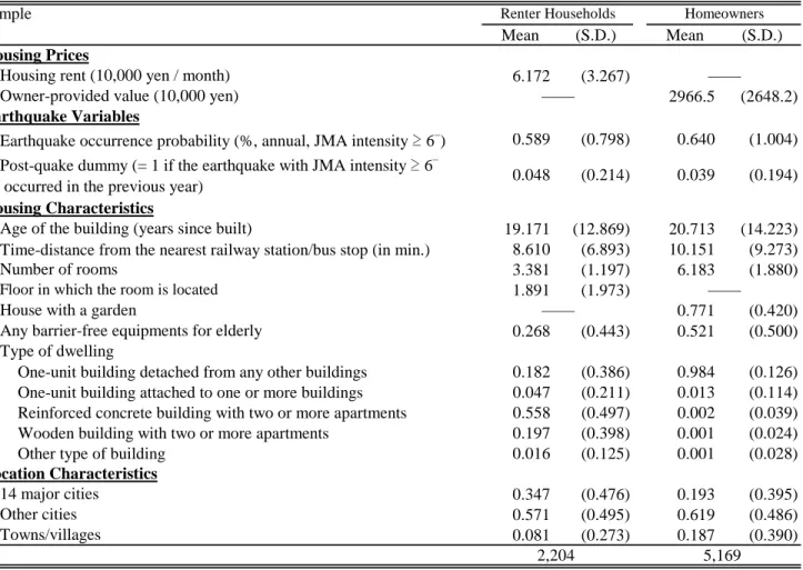
sector, self-employed, and not employed), and annual earnings.13 The definition and summary

statistics of the variables are shown in Table 1.

(Table 1 around here)

Our primary interest is in the estimate of



in equation (8), which is the post-quake change in the effect of earthquake risk on housing prices. Since the overall effect of the

earthquake risk variable on housing prices is expected to be negative, a negative estimate on



indicates that a massive earthquake and resulting damages in the prefecture increases residents’

awareness of earthquake risks.

In equation (8), the household fixed effect



_i is particularly important for two reasons. First, households living in quake-prone areas are likely to have “self-protection” for their

13 _{Since respondent’s sex and education are time-invariant characteristics, they are not included in some}

17

dwellings, e.g., seismic retrofitting. Since we cannot observe the quake-resistance quality of the

dwelling and such a characteristic should be included in housing prices, ignoring

“self-protection” behavior could cause an underestimation of the effect of earthquake risk. In the following analysis, we assume that the quake-resistance quality of the dwelling is constant

across time and can be captured by



_i in our model.14 Second, the heterogeneity of attitudes toward risk might be another problem. Less risk-averse households tend to live in quake-prone

areas. At the same time, it is also likely that these households will live in areas that have other

unobservable risky characteristics (e.g., flood hazard). In such cases, the estimated coefficients

of the model without the household fixed effect would be biased.

The possibility of another source of bias in our implicit price estimate stems from the

discrepancy between subjective and objective assessments of earthquake risk. Following the

recent study by Kniesner et al. (2007), we check this problem by using the familiar

measurement error framework. Let PR_ito be the objective estimate of earthquake probability

and PR_its be the subjective risk perception. We assume that the relationship between objective

probability and subjective risk perception can be represented as:

, it o it s it PR PR  



(9)

where



_it represents measurement error pertaining to the household’s perception toward objective risk. As shown in Section 3, the existence of the transformation bias, i.e., g_s 1, would result in faulty MWP estimate using the objective probability measure. If there is no

14 _{We do not distinguish between household and housing unit fixed effects here. Strictly speaking, since}

some households changed their residence during our sample period, these two effects are not exactly the same. In consideration of this point, we also estimated the model using a restricted sample of non-movers. However, the result does not change qualitatively.

18

measurement error (i.e.,

v

_it



0

), equation (9) immediately suggests that each household has “correct” risk assessment, and hence there is no transformation bias, g_s 1.

Instead, if there are certain discrepancies between objective probability and subjective risk

assessment as in equation (9), the implicit price in terms of objective probability might be

biased. Since our final goal is to obtain the true MWP estimate in equation (7), i.e., the implicit

price for the subjective perception, the underlying model can be written as:

 

.

ln p_it 







PR_its



EQ_itPR_its X_it







_i



_t



_it (10) If we can observe the subjective risk measure PR_its, equation (10) gives the implicit price for

the subjective risk perception, and therefore the true MWP estimate given in equation (7).

However, since we do not have any direct measure for PR_its, equation (10) cannot be estimated

in general. Instead, consider the regression of

ln

 

p

it on the observed o it

PR . By substituting

equation (9) into equation (10), we have

 









,

ln

it t i it o it it o it it t i it it o it it it o it it

X

PR

EQ

PR

X

PR

EQ

PR

p







































































(11)

where

 

_it is the combined error term equal to



_it 



_it 



EQ_it



_it. Because PR_ito

equals PR_its v_it, the regressor in equation (11) is correlated with the combined error term: .

0 ] , [

Cov PR_ito



_it  Hence the OLS estimates of equation (11) with observed PSHM (objective) probability become inconsistent and we need to use the instrumental variables method.

In this case, in order to obtain consistent estimates, we need to have valid instruments that

are: (i) sufficiently correlated with objective probability PR_ito, while (ii) independent of the

19

a subjective assessment of PR_kts . Then, equation (9) suggests that we have kt o kt s

kt PR

PR  



for this household. If the measurement error for each household is purely idiosyncratic, then we

expect that household k’s measurement error



_kt, and thus PR_kto , will be independent of household i’s



_it.15 This allows us to use neighborhood objective probability as the instrument for PR_ito. In the following analysis, we will use within-city variation of the objective

probability as our instrument, rather than picking up a single neighborhood probability

associated with a particular location.

5. Empirical Results

In the following analyses, we estimate separate hedonic regressions for renter households and

homeowners.16 Corresponding dependent variables of these two regressions are the logarithms

of monthly rents and owner-provided house values.17 We first estimate the model without the

interaction term



EQ

_it



PR

_it



to get our baseline result, and then estimate the full model given in equation (8).

15 _{One may think that people in nearby locations may have similar components in their measurement}

errors due to unobserved location characteristics or some form of residential sorting. But if such components are time-invariant, within-difference transformation of our hedonic regression can solve this problem.

16

Since our analysis is the first study to focus on both homeowners and renters’ response to massive earthquakes in one paper, we cannot expect that both renters and owners react similarly based on previous research. This is the reason why we separately estimated two equations for renters and owners.

17 _{As Kiel and Zabel (1999) and Freeman (1979) have shown, the use of the owners’ valuations will}

result in accurate estimates of house price indexes and will provide reliable estimates of the implicit prices of housing and neighborhood characteristics.

20

Baseline Results

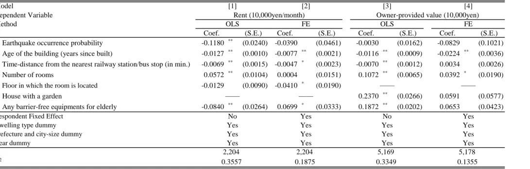
Our baseline result is shown in Table 2. Here we do not distinguish between observations before

and after the massive earthquakes. For both renter households and homeowners, we estimate the

model with OLS and fixed effects. Models [1] and [3] are OLS results without considering

household fixed effects



_i . Models [2] and [4] are fixed effects results. Respondent characteristics, and dummy variables for the dwelling types, prefectures and city-sizes are also

controlled, but omitted from the results. We have included the time dummy variables to capture

the unobserved time-varying effects that change year by year such as a housing market changes

after the earthquake.

(Table 2 around here)

For renter households (Model [1]), the OLS results indicate that earthquake probability has

a significantly negative effect on housing rents. This is consistent with previous studies (Naoi,

Sumita, and Seko, 2007; Nakagawa et al., 2007). Based on the fixed effect estimates (Model

[2]), the coefficient of earthquake occurrence probability is still negative, but not significant.

Our interpretation here is that the OLS estimate may pick up unobservable household

heterogeneity or some location-specific characteristics. For example, risk-averse renter

households may choose better houses that are located in an area with good environmental

characteristics (such as low earthquake probability, good schools or transportation links, parks

or other amenities, etc.). Without controlling for fixed effects, such an unobserved relationship

may yield a spurious negative correlation between housing prices and earthquake probability.

Statistically, the F test for the fixed effects model significantly rejects the null hypothesis of no

individual effects (

Pr



F



830

,

1223





15

.

97





0

.

000

).

For homeowners (Models [3] and [4]), the negative effect of earthquake probability

21

that the fixed effects model could exacerbate attenuation bias due to measurement errors relative

to OLS if the autocorrelation in unobserved subjective perceptions is large enough relative to

that in measurement errors (Wooldridge, 2002, p.311).18 Hence we expect that the measurement

error problems do not play a dominant role in explaining the changes in implicit price estimates

between these two models. Our intuition here is that extensive “self-protection” behavior among homeowners, which is not likely to be the case for renters, underestimates the coefficient in

OLS result.

For other independent variables, the results are intuitively plausible. Age of housing and

minutes from the nearest station/bus stop both have negative and significant signs except for the

latter in Model [4]. Number of rooms, which is used to measure the scale of housing, has a

significantly positive impact except for Model [2]. Barrier-free equipment has positive signs in

homeowner results (Model [3]). As for the renter sample, this variable has the completely

opposite sign without controlling for fixed effects (Model [1]), but it turns out to have a positive

effect in the fixed effects model (Model [3]).

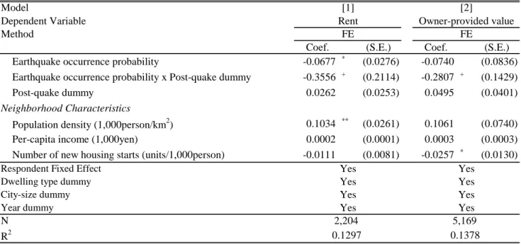
Effects of Earthquake Risk Before and After Massive Earthquakes

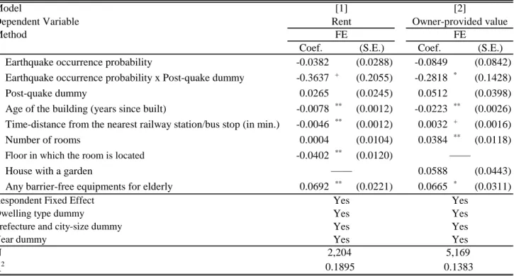
The main results of our hedonic regressions are shown in Table 3. Specification of the models

shown in Table 3 is identical to those in Table 2 with one exception; we added an interaction

term between the earthquake probability variable and a post-quake dummy variable.19 A

18

Strictly speaking, the argument can only be applicable to the fixed effect first-difference (FD) estimator, while our estimation method here is a standard within-difference estimator. With a longitudinal data of T > 2, estimates from these two fixed-effects estimators can be different. So we have also estimated the Model [2] with FD method, and find that this yields an even larger effect of earthquake probability.

19 _{If there is market segmentation, the hedonic price function estimated for large areas as a whole will}

provide faulty estimates of the implicit prices. To see whether this is the case, we also estimate the model with a selected subset of our sample (i.e., households in northern Japan). The estimation with the

22

post-quake dummy variable equals one if the earthquake event occurred in the previous year and

zero otherwise.20

(Table 3 around here)

It is found that post-quake changes in the effect of earthquake risk probability (i.e.,

coefficients on an interaction term,



) are significantly negative for both models. This suggests that massive quakes in neighboring cities/towns changed the perception of earthquake risk for

both renter households and homeowners. Our results indicate that, in the post-quake period, a

0.2 percent increase in the annual earthquake probability, which is nearly 1/3 of the average

probability, leads to a 10,000 yen discount in monthly rents and a 3.8 million yen discount in

housing values. These numbers are approximately 16% of average rent and 13% of housing

value. Moreover, our results also indicate that the pre-quake coefficients of the earthquake risk

variable are not significant in both models. Combined with the significantly negative

coefficients of the interaction terms, we believe that the most plausible interpretation for this

result is that households are initially unaware of, or at least underestimate, the earthquake risk in

the pre-quake period. The perception of earthquake risk for both renter households and

homeowners, however, changes dramatically following a massive quake in neighboring

cities/towns.21

restricted sample, however, shows qualitatively similar results.

20 _{We also introduce a post-quake dummy variable itself as an additional explanatory variable.} 21

An anonymous referee kindly suggested another interpretation for the insignificant coefficient estimates of the earthquake risk variable in both the rent and house price models as follows. With any anti-seismic construction, the value of the property before the occurrence of the earthquake will increase compared to the value of the property without any anti-seismic construction. In this sense, anti-seismic construction has a direct effect on losses and thus on the value of the property. However, anti-seismic construction may also lower the risk of a loss. Because of the latter effect, as a result, the coefficient estimates of the earthquake risk variable in both the rent and house price models become insignificant. Such a story may be plausible if anti-seismic construction is prevalent in the housing market. In Japan, however, the overall percentage of dwellings with anti-seismic construction features exceeding the

23

Several Robustness Checks

As we discussed in Section 3, the implicit price in terms of objective probability might be

biased if there are certain discrepancies between objective and subjective risk assessments. In

order to empirically check this problem, we utilize a familiar measurement error framework and

re-estimate the model using the fixed effects instrumental variables estimator for objective

probability (see Section 4 for detail). The instruments we used are the standard deviation of

earthquake probabilities at the city/town-level (within-city S.D. of earthquake probability) and

its interaction with the post-quake dummy variable. As explained before, the rationale for this

choice is that, once household fixed effects are controlled for, a particular household’s measurement (or perception) error is likely to be uncorrelated with its neighbor’s. Hence this variable should correlate with the objective earthquake occurrence probability, but is

uncorrelated with the measurement error itself.

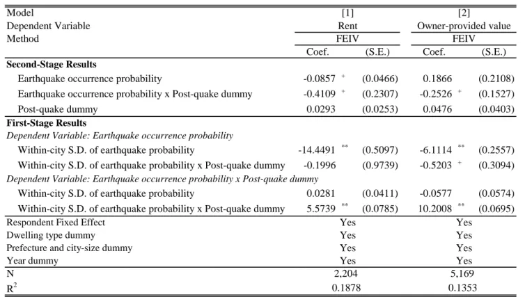
These estimation results are summarized in Table 4. The set of explanatory variables used

in the model is identical to that of Table 3. In this model, in contrast, the earthquake occurrence

probability and its interaction with the post-quake dummy are instrumented. Various housing

characteristics and other control variables are also included in the model, but are omitted from

the results.22

(Table 4 around here)

regulatory minimum is less than 3% (Housing and Land Survey, 2003).

22 _{Housing characteristics included are as follows: age of the dwelling (years since built), time-distance}

from the nearest public transportation, number of rooms, floor in which the room is located (for condominium units), whether the unit has a garden (for owner-occupied houses), whether the unit has any barrier-free equipment, and dummies for the type of dwelling. The complete results are available upon request.

24

The results of the first stage regressions are shown in the bottom part of Table 4. It is found

that the within-city S.D. of the earthquake probability is significantly and negatively correlated

with the average probability for both renter and homeowner samples. The interaction term of the

within-city S.D. is also shown to be a highly significant predictor of the instrumented

interactions for both models. These results indicate that our instrumental variables have

sufficiently strong correlation with earthquake occurrence probability and its interaction with

the post-quake dummy variable.

The second stage regression results related to earthquake occurrence probability are shown

in the upper part of Table 4. Again, the post-quake changes in the effect of earthquake

probability are significantly negative for both models. Moreover, even after controlling for

measurement errors, estimated post-quake coefficients and the implicit price estimates are

virtually identical to those presented in Table 3. To see whether measurement error problems

yield significantly different parameter estimates, we test the equivalence of the results in Tables

3 and 4 by Hausman specification tests. For the renter sample, the test statistic of 1.78, which

follows



2

 

36

under the null hypothesis, is small enough to accept the null hypothesis. For the homeowner sample, the test statistic of 2.10, which follows



2

 

22

, is also small enough

to accept the null. Hence we can say that our main results using objective PSHM probability as

a proxy for subjective risk assessment provide sufficiently reliable implicit price estimates.

As well as the measurement error issue, the main results in Table 3 rely on the assumption

that our post-quake dummy variable credibly picks up purely informational effects of the

earthquake occurrence. Because a massive earthquake will have a devastating impact on the

local housing market, it may affect housing prices through changes in overall demand and

supply conditions.23 We have already shown in Table 3 that the post-quake dummy variable

25

itself does not have any significant effects in hedonic regressions, implying that the actual

earthquakes under consideration do not have any direct impact on the local housing market.24

However, to examine this point in more detail, we added several neighborhood variables into

our regressions. In Table 5, three neighborhood characteristics are added: Population density,

per-capita income, and the number of new housing starts.25 The first two variables are expected

to control for the fact that regions with dense population and/or economic activities might suffer

much more extensive damage from a major earthquake. The number of new housing starts

would control for the changes in demand and supply in the local housing market due to temporal

shocks after a massive earthquake.

Even after controlling for these possible neighborhood effects of a massive earthquake, our

pre- and post-quake implicit price estimates are still comparable with those in Tables 3 and 4. In

Model [1] for renter households, both pre- and post-quake effects of earthquake occurrence

probability become significantly negative, and higher population density leads to higher rental

prices as expected. In Model [2] for owner households, the post-quake effect of earthquake

probability is still significantly negative with similar magnitude as those shown in the previous

results. The negative coefficient on the number of new housing starts suggests that post-disaster

on the housing market in terms of changes in house prices and housing rents and analyzed the mechanism of those changes.

24 _{An anonymous referee kindly suggested another explanation for the positive (but insignificant)}

coefficient estimates of the post-quake dummy variable. If stringent anti-seismic construction codes were adopted following the earthquakes, this policy change would lead to costly housing construction, and hence have a positive impact on the price of individual housing units. Following his/her suggestion, we have checked the recent revision of the anti-seismic construction codes in Japan. We find that there are no major revisions during our sample period.

25 _{All three variables are defined at the prefecture-levels and calculated using the following sources.}

Population density: “Annual Report on Current Population Estimates” (Statistics Bureau). Per-capita income: “Annual Report on Prefectural Accounts” (Cabinet Office). Number of new housing starts: “Annual Statistics on Construction” (Ministry of Land, Infrastructure, and Transport).

26

supply increases drive down local housing prices.

(Table 5 around here)

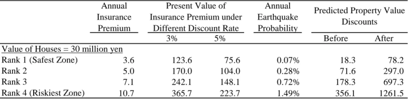
Comparing Property Value Discounts with Capitalized Insurance Premiums

We compare the predicted property value discounts with the present value of earthquake

insurance premiums in Table 6 based on our results in Table 3 to investigate whether

homeowners alter their subjective assessments of earthquake risks after massive earthquakes

under the partial coverage insurance. As discussed in Section 3, if homeowners are

well-informed about earthquake hazards and are fully insured, property value discounts along

with the increased earthquake risk should be equal to the negative of the premium increment,





r

p





. In reality, however, since earthquake insurance only covers damages and losses of housing assets and family items, earthquake risk has some components, such as injury, death,

and some non-monetary losses, that cannot be insured. Hence we expect that housing price

reductions might exceed the cost of earthquake insurance, that is, we expect

p

_



r

_



0

where

p

_



0

and

r

_



0

. The purpose of Table 6 is to examine whether

p

_



r

_, the uninsured component of earthquake risk (i.e., the household’s true MWP under the partial

coverage insurance case), changes after massive earthquakes.

Since most renter households in Japan do not take out earthquake insurance, we primarily

focus on homeowners and owner-provided housing values. For the calculation of earthquake

insurance premiums, we assume earthquake insurance for a house with a value of 30 million

yen.26 Annual insurance premiums are based on NLIRO insurance rates for wooden housing

without any anti-seismic construction method. Since annual insurance premiums basically

depend on the earthquake hazard of the area in which a house is located, we estimate the

27

premiums for four risk categories (Rank 1 (safest zone) – Rank 4 (riskiest zone)). The annual

insurance payments are discounted using discount rates of 3% (column 2) and 5% (column3).

For the calculation of property value differentials, we use the housing value discounts from

a hypothetical riskless situation (i.e., earthquake probability = 0%). Based on the observed

average earthquake probability for each risk category (column 4), predicted house values are

calculated and the property value discounts are obtained. Property value discounts are defined as

the predicted property value under a riskless situation minus that under an actual earthquake

probability. Hence the property value discounts presented here can be interpreted as an

empirical counterpart of the implicit price for the earthquake probability in absolute terms, i.e.,



p

. We calculated these property value differentials for both before and after the earthquake

event (columns 5 and 6).

(Table 6 around here)

When we look at the insurance premiums under a 3% discount rate, property value

differentials for the pre-quake period are smaller than insurance premiums except for risk

ranking 4, which means

p

_



r

_ and hence

p

_



r

_



0

. Given that the Japanese insurance system does not provide full coverage, this is counterintuitive since, if

p

_



r

_



0

, equation (7) implies that the consumer has higher utility when the earthquake occurs. A possible

interpretation is that pre-quake assessments of

p

_ are underestimated, i.e., homeowners are

initially in denial about earthquake risk. Assuming a 5% discount, we can say the same thing

except for risk rankings 3 and 4. The post-quake discounts, on the other hand, generally exceed

the capitalized insurance costs, i.e.,

p

_



r

_



0

. These results are consistent with above interpretation that homeowners initially underestimate the earthquake risk before an actual

28

than pre-quake assessments, the difference between post-quake property value discounts and the

present value of insurance premiums represents the uninsurable cost of earthquakes.

6. Conclusion

The purpose of this paper is to examine whether individuals alter their subjective assessments of

earthquake risks after massive earthquake events. We use nation-wide household longitudinal

data coupled with earthquake hazard information and the observed earthquake record to

estimate individuals’ valuation of earthquake risk. The earthquake risk premium is estimated using hedonic price models for housing rents and owner-provided house values. Using a

difference-in-differences (DID) approach with longitudinal data, we find that there are some

modifications of individuals’ assessments of earthquake risk following a major tectonic event. Our results for homeowners suggest that the post-quake discounts for property values within

quake-prone areas more than doubled compared with pre-quake values. We argue that the most

likely interpretation for this result is that homeowners initially underestimate earthquake risk.

The policy implication of our results is clear. If the government properly assesses

earthquake risk and this assessment is widely disseminated among the public, occurrence of

earthquake events would not substantially alter individuals’ perception toward risk. In this paper,

however, we find evidence of significant changes in risk assessment resulting from the actual

experience of massive earthquakes. Our results indicate that there is much room for

improvement in current anti-seismic disaster policies regarding public perceptions of potential

earthquake losses.27

27 _{Quigley and Rosenthal (2008) show the importance of a diverse treatment of the economic and public}

aspects of urban disasters. Troy and Romm (2006) assess the effects of hazard disclosure on housing prices in statutory flood- and fire-hazard zones and analyze whether those effects were conditioned by

29

Improved risk assessment depends on the government’s extensive educational campaigns and greater transparency concerning the government’s local risk assessments. In addition, the earthquake insurance system should be modified by the government to reflect more precise risk

assessment. If the earthquake insurance system truly reflects more precise earthquake risk

assessment, and the results are widely disseminated, households are more likely to recognize the

true extent of earthquake risk in their own areas and act accordingly.28 In order to increase

consumers’ awareness of natural hazard risk, introduction of a law for housing lenders, sellers and real estate agents requiring disclosure of natural hazard risk, such as the 1998 California

Natural Hazard Disclosure Law (AB 1195)29, might be an effective policy. It is important to

remind households to always properly assess earthquake risk even if they have never

experienced massive earthquakes in their areas, and these reminders are most likely to be

effective at the point of sale, i.e. real estate brokers and housing lenders. Our results suggest that,

prior to massive earthquakes, homeowners tend to underestimate earthquake risk, or are totally

unaware that they live in a quake-prone area, and thus do not adopt adequate anti-seismic

measures or purchase insurance policies. This lack of awareness justifies some form of

government intervention regarding anti-seismic policies that help people better assess and

address their risk.

The government should devise anti-seismic policies reflecting accurate earthquake risk

assessment in each area. For example, the government should impose strict anti-seismic

building codes for buildings in risky areas and encourage households to modify their dwellings

to lessen seismic risk. Targeted subsidies and tax deductions aimed at promoting seismic risk

race/ethnicity, income, and previous occurrence of hazards in those zones.

28 _{Kunreuther (2008) examined the role that insurance and mitigation can play in reducing losses from}

natural disasters.