Studies on hydraulic environments in the Khung Kraben bay, eastern Thailand-香川大学学術情報リポジトリ

Tech.. Bull. Fac.. Agr.. Kagawa Univ.,Vol. 37, No. 1, 55-.65, 1985

S T U D I E S ON HYDRAULIC E N V I R O N M E N T S IN T H E KHUNG K R A B E N

BAY,

E A S T E R N THAILAND

Takashi

SASAKI

and Hiroo Inoue

A series of field surveys on the development and conservation in the coastal brackish zone of Thailand were carried out by the Thai-Japanese Joint Research Project Group in December, 1983.

This i s the report on the results of investigation and simulation of the hydraulic characteristics of the Khung Kraben Bay located in the eastern Thailand

The simulation techniques on patterns of sea water flow were checked on the basis of field data observed in the bay Changes in discharge and water volume were evaluated

It was found that if the volume of inflow from the mouth of the bay is Qe and the water volume a t

L

W i s V1, then the exchange rate of sea water,

Qe/

Vl

i s 6 0 in 1/24 hrs.

Introduction

The second field survey on the development and conservation in the coastal brackish zone of Thailand was carried out by the Thai-Japanese Joint Research Project Group in December, 1983. The location

investigated was the Khung Kraben Bay near Chantaburi, which is surrounded by a mangrove forest. The main target to be pursued was an assessment of the possibilities for fisheries development in the Khung Kraben Bay.. We took partial charge of a series of ecological studies by carrying out the investigations on hydraulic characteristics, water quality and bottom-sediment properties in the bas..

56

Tech Bull Fac Agr Kagawa Univ ,Vol 37, No 1, 1985

Method

1 Field observation

During the period from Dec 9 to 23, 1983, observations were carried out in Ao Khung Kraban, located in eastern Thailand At each station shown in Fig 1, current velocity, water temperature and salinity were measured a t 1 5 m below the surface Flow patterns were also investigated by noting the movements of drifters over a given time in the bay Measurement of water level was made a t the mouth (Stn X )

Main instruments used were a depth/temperature meter (TECNA E L E C I R O CO ), a portable water current meter with compass (MODEL 201, MARSH & MCBINEY CO.), a salinometer (SCT, YSI-33, YELLOW SPRINGS Inst C o ) and a portable recorder (TYPE 3057, YOKOCAWA ELECTRIC WORKS C O ) .

Fig..l Observed trajectories of drifters.

Table. 1 Movements of d r i f t e r s with time a t ebb tide, Dec. 20-21, 1983. (See Fig.. 1) Drifter 1 2 3 4 5 6 7 8 9 N a l 1 1216 1358 1456 1552 1610 lh2 1 1215 1358 1456 1555 h m N a 3 1035 1053 1202 1352 1435 1535 1617 1706 1730 h m N a 4 1030 1107 1157 1352 1430 1530 h m 1130 1245 1332 1510 1608 1645 1725 h m N a 6 1125 1220 1350 1515 1605 1652 h m l h 7 1123 1125 1220 1340 1520 1600 1655 1 1155 1310 Dec,20,1983 Dec.21.1983

T.

SASAKI

and H.

INOUE

: HYDRAULIC ENVIRONMENTS

2 Numerical simulation

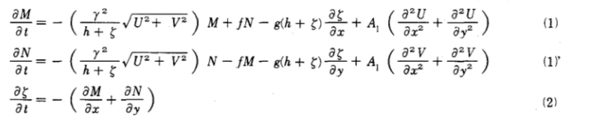
The equations for horizontal motion of homogeneous fluid, averaged vertically and neglecting the convective term and the equation for continuity a r e formulated a s follows :

where t i s the time,

5

the water level displacement of the free surface from its mean level, (4 ,y) the horizontal cartesian coordinate, and

(U,

V) the horizontal component of velocity in the ( ~ c , y ) direction.. _{A l} is the coefficient of horizontal eddy viscosity, y the coefficient of bottom friction, f the Coriolis parameter and g the acceleration due to gravity, respectively..

( M , N

i s defined a s follows:

where (uv) is the velocity in the ( L , ~ ) direction at z,h the local mean water depth, and z the depth from the mean water -level, respectively

Table 2 The parameters related to the computer simulation

Discr iption Unit 'Symbol Value

time interval s e c A t 14

grid interval cm hs 10000

acceleration of gravity cm/sec g 980 horizontal eddy viscosity cm2/sec A, 6840

bottom friction y 0 0052

Coriolis parameter l / s e c f 0 00003

Fig.2 Analysis area for the finite-difference method with square meshes.

58

Tech. Bull. Fac.. Agr. Kagawa Univ,,Vol. 37, No 1 , 1 9 8 5

In addition to these equations, i t i s necessary to prescribe initial data and boundary data to have a completly formulated problem with difinitely determined solution A s initial data we must have, a s i s to be expected, the values of stage and the velocity a t some instant of time chosen a s initial time a t which calculation i s to begin Boundary data a r e required a t the mouth of the bay under consideration

T h e s e equations w e r e solved by a finite-difference method with horizontal square meshes (Fig.2) T h e computer program presented by T o UENO (1971)(') was modified for use in the present study Various parameters related to the computer simulation a r e shown in Table.1

Using these numerical solutions obtained with the aid of a high speed digital computer, the Lagrangian movements of a certain mass of water a r e estimated by use of the following equations :

d

=

j:

Udt

where ( d t ) , y(t)) i s the distance traveled from the origin

In E q (4) (U, V) can be obtained by solving numerically E q s (1) and (2) But the d r i f t e r s under consider a - tion do not always stay a t any particular time on the grid point possessing the velocity (UlV1, VlS1) Therefore, practical formulations of E q (4) may be rewritten for the computation a s follows(2)

:

where

x ,

Yf:

: the horizontal distance traveled from the origin a t the end of each time frame (n) Here,n = 0, 1 , 2, 3,

."

".

A t : the time frame

Uk, Vk : the horizontal velocity a t each poisition

(hl)

with reference to grid points (i, j)

Using the velocity ( U l j , Vij) a t the (i,j) grid point for the tidal c u r r e n t s simulation, the velocity (Uk, Vk) a t any place i s represented on the basis of Taylor's theorem a s follows

:

T..

SASAKI and H.. INOUE : HYDRAULIC ENVIRONMENTS

59

In applying Eq (51, i t i s necessary to give the coastal line boundaries In this paper, seven types of boundaries a r e assigned a s shown in F i g 3

: sea

0

: land

60

Tech. Bull. Fac. Agr.. Kagawa Univ.,Vol.. 37, No.. 1, 1985

Result and discussion

The results of the observations a r e shown in Figs 1 and 4-6 Fig 1 shows the Lagrangian movements of the particular water mass. From this figure, the circulation pattern in the bay is seen generally counter- clockwise a t ebb tide The motion of sea water in the bay was almost entirely controlled by the inflow from the mouth of the bay, since inflow from the local canals was quite small

The water levels were measured a t S t n

X,

Dec 11-12, 18-19, 20, 21, and 22, 1983 (Fig 4). As shown in F i g 4 , the tide was regular diurnal a t S t n X The difference in water levels between successive high and low waters was 128.7 cm a t spring tide in Laem Sing (ROYAL THAI NAVY, 1983) Tide currents, salinity and water temperature were measured at S t n

X,

Q and P The results a r e shown in F i g 5 and F i g 6 The maximum value of velocity was 41 0 cm/sec a t ebb tide, Dec 22, 1 9 8 3 The salinities and temperatures were 30.0- 3 3 1 % O and 25 5 - 29 0 ° C at Stn

X,

28 8 -31 7 % O and 26 1 - 2 7 5 "C a t Stn.. P,and 32 9 - 29 0 % O and 27 3

-

28 0 "C a t S t n Q

TIME OF DAY

F i g 4 Variations in water temperature and salinity a t depth 1 5 m below the sea surface, and tide curve Measured a t Stn. X, Dec 18-19, 1983

Fig..5 Current speed and direction a t depth 1 . 5 m below the surface.. Variations in water temperature and salinity a t depth 1 . 5 m below the sea surface. Measured a t Stn..

X,

Dec. 13, 1983.

U VI \ Z

_ - - _

_ - - -

30 26 W

a

'O 29 25 Crl 3 28 24 U I 10 11 12 13 14 15 16 17 TIME OF DAY 180

-

(S )

'

90

9

k

( y .

g

(N)

5

YO a (F:) I80 (s) 10 11 12 1.3 14 15 16 1 7 TIME OF DAY - - ' I I - L k Crl Z W

3

2

cn 5

T . SASAKI and H. INOUE : HYDRAULIC ENVIRONMENTS

1124 1214 1304 1354 1444 1534 1624 1744

TIME OF DAY 180

(S:

I

Based on the observed data, the distributions of tidal c u r r e n t s in the bay, which a r e calculated with the aid of a digital high speed computer, a r e shown in F i g 7 F i g 8 shows variations in tidal c u r r e n t and tide level over a period of time in some selected positions in the bay

Using the distributions of c u r r e n t s obtained by the digital computer simulation, Lagrangian movement of water m a s s over the tidal cycle was checked a s shown in Fig.9.

I t can bc seen that the drifter trajectories obtained by field observations ( F i g 1) w e r e essentially similar to those computed, from a macroscopic standpoint.

i 90

2

"I" 0 .

y

(N) 90 (E)

Fig.7.a Distribution of tidal curents during flood tide ; 4 hours before high tide.

-

. .

-

Fig.7.b Distribution of tidal c u r r e n t s during ebb tide ; 1 hour before high tide

180

($1 1124 1214 1304 1354 1444 1534 1624 1744

TIME OF DAY

F i g 6 C u r r e n t speed and direction a t depth 1 5 m below the s e a surface Measured a t S t n P, Dec 22, 1 9 8 3

Tech Bull F a c Agr Kagawa Univ ,Vol 37, No 1, 1985

F i g 7 c Distribution of tidal c u r r e n t s during ebb tide ; 2 hours

after high tide

F i g 7 d Distribution of tidal c u r r e n t s during flood tide ; 5 hours after high tide

F i g 7 e Distribution of tidal c u r r e n t s during ebb tide ; 4 hours before low tide

F i g 7 f Distribution of tidal c u r r e n t s during ebb tide ; 1 hour before low tide

T . SASAKI and H.. INOUE : HYDRAULIC ENVIRONMENTS 0. 5 I D 1 5 20 25 3 0 3 5 UO I ' _ T I D A L C U R R E N T I N - K H U N G K R A B E N B A Y 6PRIND TIDE T I N E 1 2 1

-

1DO<*,.rr

Fig.7.g Distribution of tidal currents during flood tide ; 2 hours

after low tide.

Fig..7.h Distribution of tidal currents during flood tide ;

5

hours , after low tide.

Once the tidal current and the tidal level have been coded for a computer, it becomes possible to solveall s o r t s of hydraulic problem quickly.. In the present study, changes in discharge and water volume were evaluated. The hydraulic characteristics a r e summarized a s shown in Fig. 10 and Table.3..

It may be found from Table 3 that a s the volume of inflow from the mouth of the bay i s Qe and water

volume a t L..W. i s Vl, the exchange rate of sea water Qe/ Vl i s 6.0124 h r s

...

This means that 86 % of the volume of the bay water a t low water i s replaced with open sea water, in one tide cycle.

Table 3 Hydraulic characteristics in Ao Khung Kraben near Chantaburi.

Exchange r a t e Q e '

5

1 / 24hr 5 9 Remarks c y c l e 1 Volume of inflow Qe m3/ 24hr 130 X 10' vh/

v~

5 3

Water volume, m 3 Volume of

outflow Q o m3/24hr 135 X loG L W

5

22 6 X loG H W vh 120 0 X 10'

Tech.. Bull. Fac.. Agr. Kagawa Univ ,Vol. 37, No.. 1, 1985

KHUNG K R A B E N B R Y S T A T I O N 8

L

T I D E I B P R I N G P E R I O D 0 H A 8 T O 2 5 H R 8 AT G R I D P O I N T t O L [ 9 0 . 1 4 ) H R 8 I - 7 T - ' Y ' 4 ' 5 ' B - 7 P B 1 § - I U 7 i I l 1 T i 5 7 4-'I S 7 1 E 7 1 T 1 ELEVA'TI ON * l o 0 CH T I D E 1 8 P R I N G P E R I O D 0 H R 8 T O 2 5 H R 8 AT G R I D P O I N T 1 R L ( 3 0 . 151 H R 8 ~ ~ ' ~ T - I z T ~ T ~ I T ? ~ , - I 0 0 CH

T. SASAKI and

H..

INOUE : HYDRAULIC ENVIRONMENTS

Fig.,9 Computed drifter (water mass) trajectories..

Variations in tidal discharge and water volume in the Khung Kraben

Acknowledgements

We wish to thank Dr. M. Bhovichita, Mr.. U.. Sittiphuprasert and Mr..

P..

Chotipuntu of the Faculty of Fiseries, Kasetsart University in Thailand, for helping in our field surveys. Thanks a r e also due to Mr. K.. Chalayondeja and Mr.. S. Limsapul of the Brakishwater Fisheries Division in Thailand, who gave valuable assistance in various ways. The.. computations in this paper were carried out on a MELCOM- COSMO-700s in the data station of Kagawa University. The authors would like to thank their staffs and Mr. Yoshihiko Tsuruta, a graduate student, for their cooperation in the present study.

References

(1) T.. UENO : Bulletin of the Kobe Marine (2) S..UMEL) \ , ~ I I ( I u t h e ~ s : Proceedings of Coastal Observatory, No.187, 1-88 (1971). Engineering in Japan, 25th, 538-542 (1978).