Okayama University Scientific Achievement Repository http://ousar.lib.okayama-u.ac.jp/54460
SOUND COLLECTION SYSTEMS USING A CROWDSOURCING APPROACH TO CONSTRUCT SOUND MAP BASED ON SUBJECTIVE EVALUATION
Sunao Hara, Shota Kobayashi and Masanobu Abe
Copyright © 2016 IEEE. Reprinted from EEE ICME Workshop on Multimedia Mobile Cloud for Smart City Applications (MMCloudCity-2016). This material is posted here with permission of the IEEE. Permission to reprint/republish this material for advertising or promotional purposes or for creating new collective works for resale or redistribution must be obtained from the IEEE by writing to [email protected] . By choosing to view this document, you agree to all provisions of the copyright laws protecting it.
SOUND COLLECTION SYSTEMS USING A CROWDSOURCING APPROACH TO
CONSTRUCT SOUND MAP BASED ON SUBJECTIVE EVALUATION
Sunao Hara, Shota Kobayashi and Masanobu Abe
Okayama University
Graduate school of Natural Science and Technology
3-1-1, Tsushima-naka, Kita-ku, Okayama, Japan.
[email protected]
ABSTRACT
This paper presents a sound collection system that uses crowdsourcing to gather information for visualizing area characteristics. First, we developed a sound collection sys-tem to simultaneously collect physical sounds, their statis-tics, and subjective evaluations. We then conducted a sound collection experiment using the developed system on 14 par-ticipants. We collected 693,582 samples of equivalent A-weighted loudness levels and their locations, and 5,935 sam-ples of sounds and their locations. The data also include sub-jective evaluations by the participants. In addition, we ana-lyzed the changes in sound properties of some areas before and after the opening of a large-scale shopping mall in a city. Next, we implemented visualizations on the server system to attract users’ interests. Finally, we published the system, which can receive sounds from any Android smartphone user. The sound data were continuously collected and achieved a specified result.
Index Terms— Environmental sound, Crowdsourcing, Loudness, Crowdedness, Smart City
1. INTRODUCTION
Data collection and analysis are key technologies for a smart city [1]. For the success of data collection in a smart city, we need to gain the cooperation and participation of residents [2]. Mobile phone sensing [3, 4] is a promising approach for res-idents to sense a city’s characteristics. Mobile phones and recent smartphones contain a rich set of powerful embedded sensors. Especially, Global Positioning system (GPS) sensors and microphones are installed on most smartphones, although the set of installed sensors varies among smartphones. Con-sequently, sound collection with location information using sensors is a hopeful approach for the success of data collec-tion with cooperacollec-tion from residents.
This work has been partially supported by Strategic Information and Communications R&D Promotion Programme (SCOPE) from Ministry of Internal Affairs and Communications, Japan.
In this study, we developed a sound collection method that uses crowdsourcing to understand environmental sounds by considering contextual information. The sound collection is performed using an Android application [5] on a smart device. The collected data fall into two types, user-specific and sta-tistical. We use two crowdsourcing paradigms to collect the sounds: participatory [6, 7] and opportunistic sensing [8]. Us-ing the participatory sensUs-ing paradigm, we can collect sounds that participants are interested in or appreciate, therefore, we used this paradigm to collect the waveforms of sounds. Us-ing the opportunistic sensUs-ing paradigm, we can collect sound statistics and, in particular, the loudness levels as statistics.
Moreover, we developed a visualization method for the sounds collected using participatory and opportunistic sens-ing. This visualization is one of the most important capabili-ties for interpreting environmental sounds. The waveforms of sounds are visualized as icons symbolizing the sounds at par-ticular locations on a map, and the statistics of the sounds are visualized as colors on the same map. We also implemented system functions that can be used for crowdsourcing-based sound collection.
2. BACKGROUND
Sound properties are generally interpreted as having spectral and/or temporal parameters, such as spectrum, fundamental frequency, and loudness. However, these parameters only in-terpret the sound properties on the basis of a common under-standing of human beings; this is insufficient. To understand environmental sounds in the real world, we need to consider contextual information, i.e., not only sound properties, but also the situation of the listener.
The data must be statistically processed or anonymized to reduce any privacy risk for public systems. From this per-spective, EarPhone [9] and NoiseTube [10] are important ex-amples. In these studies, the researchers attempted to col-lect environmental sounds as sound levels using crowdsourc-ing; in other words, they dealt primarily with the statistics of sounds. McGraw et al. [11] collected sound data using
Amazon Mechanical Turk as a crowdsourcing platform. Mat-suyama et al. [12] conducted their sound-data collection us-ing an HTML5 application and evaluated the performance of sound classifiers. Their study deals primarily with the raw waveforms of sounds, which cannot identify the listener. In contrast with these studies, the principal contribution of our paper is to enable sound-data collection that takes contextual information into account.
In this paper, we refine a system that was implemented by Hara et al. [5]. In particular, A-weighted loudness levels [13, 14] can be recorded in the application.
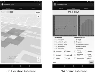
3. SOUND COLLECTION SYSTEM 3.1. Recording application for environmental sound We developed a recording application for environmental sound. We used a Google Nexus 7, a 7-inch touch screen tablet for the Android OS. Figures 1(a) and (b) show screen shots of the location- and sound-logging screens, respectively. Data recording begins when the user slides the button at the upper side of the screen.
On the location-logging screen, the system can record highly accurate location information using GPS, Cell-ID, or Wi-Fi networks via the Android API. The default sampling rate is 1 s, but the user can change this through the settings. Pin icons on a map on the screen can show the history of the user’s locations.
On the sound-logging screen, the system can record raw sound signals and calculate loudness levels using a micro-phone on the device. It always stores the sound data of the most recent 20 s using a ring buffer, and it also analyzes the sound to calculate the equivalent loudness level and the levels of an eight-channel frequency filter bank at intervals of 1 s.
Users can attach annotations, such as subjective evalua-tion, sound type selecevalua-tion, and free descripevalua-tion, to a sound while recording. The subjective evaluation uses a five-grade scale for two metrics, subjective loudness level and subjec-tive crowdedness level. The sound type is easy to annotate with a selection of five preset sound types. A free description can be used as a summary of such features as the recording environment, or feelings.
All of the annotations are recorded in log files with time information, and a WAV file including 10 s of sound is cre-ated at the same time. These can be sent to a server, if the application settings permit. The sent log files are parsed on the server and shown in a timeline view that is similar to that of Twitter, and is shared for all users in the implementation. 3.2. Specification of the data collected by the application The application generates sound files and three types of log file in one session. The log files are a location history log file, loudness level log file, and tweet log file, each containing time information, which is triggered.
(a) Location tab page
Loudness Crowdedness 1. very quiet 2. relatively quiet 3. relatively noisy 4. quite noisy 5. very noisy 1. empty 2. sparse 3. relatively crowded 4. quite crowded 5. crowded Human Birds Insects Wind Animal Cars Railway crossing Ambulance sirens motorcycles Trains Traffic signals Music
(b) Sound tab page
Fig. 1: Screenshots of Android application
Sounds are recorded at a sampling frequency of 32,000 Hz and 16 bits per second with a single channel. They are ana-lyzed at equivalent A-weighted loudness level [13, 14] Leq per second: X[k] = 1 N N −1 X n=0 x[n] · e−2πjkn/N (1) Leq= B 10 log10 1 K K−1 X k=0 A[k] · X[k] 2! (2) where x[n] is a sampled signal, N is the signal length, A[k] is an A-weighting filter, K is an FFT length (K > N ), and B(·) is a transform function from a power of quantized wave-form to a sound pressure level. In this paper, N is fixed to 32,000, which is equivalent to 1 s. B(·) is detected through a preliminary examination to compare with values of a sound level meter, RION NL–42.
The microphone specification must be calibrated appro-priately if it is to be used in a real crowdsourcing environ-ment. For this purpose, we measured sound properties and prepared B(·) functions for 22 devices. Automatic detection of the calibration parameter is future work.
In addition to Leq, this system can also record filter bank output levels in eight-channel, which is related to oc-tave band filter analysis. The filter is implemented using triangle windows. The central frequencies of the filter are fc= [63, 125, 250, 500, 1000, 2000, 4000, 8000].
3.3. Server application for collection and exploration of sounds
The client and server applications communicate via HTTP protocols. The server implements APIs for receiving and browsing data and the browsing API can create not only a general HTML view for web browsers, but also a JSON (JavaScript Object Notation) view for advanced applications.
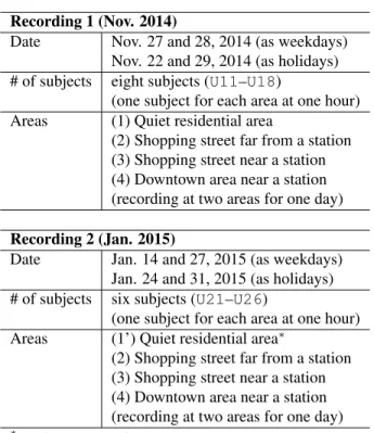
Table 1: Condition of database recordings Recording 1 (Nov. 2014)
Date Nov. 27 and 28, 2014 (as weekdays) Nov. 22 and 29, 2014 (as holidays) # of subjects eight subjects (U11–U18)
(one subject for each area at one hour) Areas (1) Quiet residential area
(2) Shopping street far from a station (3) Shopping street near a station (4) Downtown area near a station (recording at two areas for one day) Recording 2 (Jan. 2015)
Date Jan. 14 and 27, 2015 (as weekdays) Jan. 24 and 31, 2015 (as holidays) # of subjects six subjects (U21–U26)
(one subject for each area at one hour) Areas (1’) Quiet residential area∗
(2) Shopping street far from a station (3) Shopping street near a station (4) Downtown area near a station (recording at two areas for one day)
∗(1’) is another area from (1)
The server system includes several open-source software applications. The server OS is a Debian GNU/Linux 7.5 (Wheezy). The web application framework is Mojolicious1 with Perl. The back-end database software is MongoDB2. The application runs on Mojolicious Hypnotoad with an ng-inx front-end server3. The system is used for the crowd-sourced sound recordings; hence, a large number of users will use the system, and it must have the appropriate processing capacity. These software have a distributed computing archi-tecture that might provide an answer to problems of heavy usage.
4. DATABASE CONSTRUCTION 4.1. Conditions of data collection
The detailed condition of data collection is summarized in Ta-ble 1. Data was collected by a total of 14 participants at four types of areas. The participants were instructed on how to use smart devices and the data collection applications. They were asked to collect the sounds, annotations, and loudness levels. They were asked to travel around static routes for each area in 1 h. The rounds were repeated from 8 a.m. to 9 p.m.
The participants recorded loudness levels with the appli-cation running and sounds with annotations at various
inter-1http://mojolicio.us/ 2http://www.mongodb.org/ 3http://nginx.org/ 0 100 200 300 400 500 600 700 800 900 U 1 1 U 1 2 U 1 3 U 1 4 U 1 5 U 1 6 U 1 7 U 1 8 U 2 1 U 2 2 U 2 3 U 2 4 U 2 5 U 2 6 N um ber of dat a Subject ID
Fig. 2: Number of sound data as a function of a subject ID vals by the user. They held the devices in their hands dur-ing data collection keepdur-ing them in an appropriate position for collecting clear sound. However, footstep noise could be mixed in with the recorded sound, because participants might be handling the device while walking, which can cause a bias in the loudness levels.
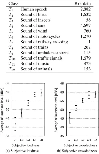
The subjective loudness level is evaluated on a five level scale: L1: very quiet, L2: relatively quiet, L3: relatively noisy, L4: quite noisy, and L5: very noisy. The subjective crowdedness level is also evaluated on a five level scale: S1: empty, S2: sparse, S3: relatively crowded, S4: quite crowded, and S5: crowded. The subjective evaluations are recorded as annotations.
The sound file containing the last 10 s of sound is cre-ated by pushing the tweet button on the sound logging screen (Fig. 1 (b)). To add an annotation to the sound, participants select the sound type before pushing the tweet button. Five types of sound are preset for ease of use and users are allowed to select multiple choices: T1: human speech, T2: birds, T3: insects, T4: cars, T5: wind, T6: motorcycles, T7: railway crossing, T8: trains, T9: ambulance sirens, T10: traffic sig-nals, T11: music, and T12: animals.
Additionally, participants can input free text to annotate the sound or recording environment. They are not required to fill in all of the selections, but can input just one part with an annotation if they want to check one or more metrics. 4.2. Summary of collected data
All of the collected data were synchronized with their time information, and we obtained 693,582 loudness data with tu-ples of latitude, longitude, and time. The sound data com-prised 5,935 collected samples with 10 s of sound with the same tuples. The number of collected data for each user is shown in Fig. 2. A distribution of the sound data collected for each type is shown in Table 2.
4.3. Analysis focused on subjective evaluations
Figures 3(a) and (b) are the average loudness levels as func-tions of the subjective loudness and crowdedness levels,
re-Table 2: Type of environmental sound and its distribution Class # of data T1 Human speech 2,882 T2 Sound of birds 1,632 T3 Sound of insects 58 T4 Sound of cars 4,697 T5 Sound of wind 760 T6 Sound of motorcycles 1,270 T7 Sound of railway crossing 1 T8 Sound of trains 267 T9 Sound of ambulance sirens 115 T10 Sound of traffic signals 1,679 T11 Sound of music 873 T12 Sound of animals 153 35 40 45 50 55 60 65 L1 L2 L3 L4 L5 Av erage of loudne s s lev el [dBA] Subjective loudness
(a) Subjective loudness
35 40 45 50 55 60 65 C1 C2 C3 C4 C5 Av erage of loudness lev el [dBA] Subjective crowdedness (b) Subjective crowdedness
Fig. 3: Average loudness level as a function of a subjective evaluation. The error bars indicate 90% confidence inter-vals as estimates of average loudness levels for the subjective level.
spectively. The average value is calculated as the average of the data from the 14 participants, and the error bars are indica-tive of 90% confidence intervals. We find overlapping error bars in Fig. 3(a) at L4and L5. Figure 3(b) has a similar ten-dency at C4and C5. This is not trivial because of the design of our questionnaire, but its long error bars show the impor-tance of listener-specific information for sound interpretation. Table 3 shows frequency for the subjective crowdedness and loudness data as a contingency table. The number of data is zero or very small at low loudness levels and high crowd-edness level, e.g., C4and L1. However, this is not the case for small values at high loudness levels and low crowdedness level, e.g., C1 and L4. This asymmetric property indicates that estimating loudness levels from a crowdedness level is much easier than estimation crowdedness levels from a loud-ness level.
Table 3: Frequency of sound data for subjective crowdedness and loudness L1 L2 L3 L4 L5 (null) TOTAL C1 390 417 221 32 3 3 1,066 C2 134 1,437 1,228 199 44 7 3,049 C3 2 111 745 241 21 6 1,126 C4 0 4 79 178 39 1 301 C5 0 0 2 26 26 1 55 (null) 9 36 52 16 4 221 338 TOTAL 535 2,005 2,327 692 137 239 5,935
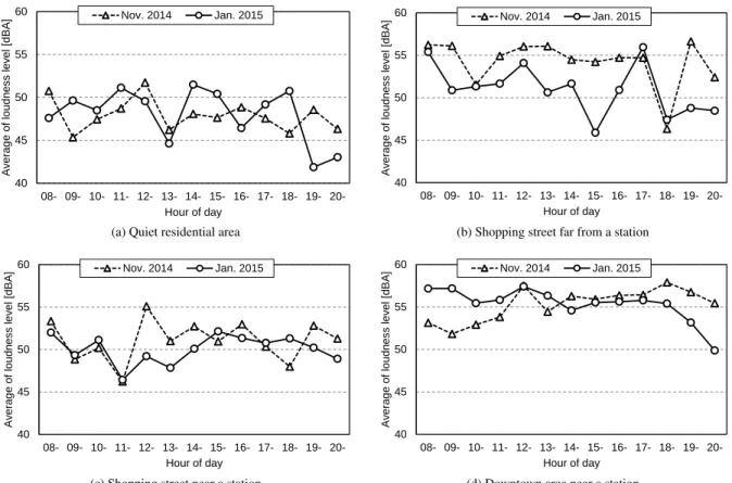
4.4. Analysis focused on the time series at hour of day Figure 4 shows time series of loudness level for each area. The sequences at a quiet residential area (Fig. 4(a)) show little difference. We can imagine that area (1), recorded on Novem-ber 2014, is noisy at night, but that area (1’), recorded on Jan-uary 2015, is quiet at night. It is vice versa from 2 p.m. to 3 p.m.
We can see in Fig. 4(d) that the loudness level undergoes a major change from night to morning. One of the reasons is the opening of a large-scale shopping mall at the beginning of November 2014. The impact of the attraction of a large-scale retail store might be what is shown in this loudness level chart. We must consider from Figures 4(b) and (c) the impact of the opening of the shopping mall on the existing shopping streets. The figure shows that there are fewer changes in the morning and evening. These are commuting times to school and work and thus show no change from before to after the opening of the shopping mall. On the other hand, it shows a non-negligible impact at noon and night. Needless to say, the charts show only that the loudness level decreases in the area. However, this might indicate that there are fewer people in the area than there were previously.
5. SOUND COLLECTION SYSTEM FOR A CROWDSOURCING APPROACH 5.1. Functionality of crowdsourcing applications
The system statistically processes loudness data with spatio-temporal indices; latitude, longitude, and time. The number, sum, and squared-sum of data for each index are calculated as a sufficient statistic of Gaussian distribution. The calculation is implemented using the Map-Reduce function of MongoDB to make scaling out the collection system easy. This scalabil-ity is important for successful crowdsourcing.
The statistics are updated on demand by uploading data from users. Users can see their contribution to the collection on our sound visualization map after a few minutes. The vi-sualization of the contribution and the quick response are also important factors in crowdsourcing.
40 45 50 55 60 08- 09- 10- 11- 12- 13- 14- 15- 16- 17- 18- 19- 20-A v erag e of l ou dn ess lev el [ dB A ] Hour of day Nov. 2014 Jan. 2015
(a) Quiet residential area
40 45 50 55 60 08- 09- 10- 11- 12- 13- 14- 15- 16- 17- 18- 19- 20-A v erag e of l oudn ess lev el [ dB A ] Hour of day Nov. 2014 Jan. 2015
(b) Shopping street far from a station
40 45 50 55 60 08- 09- 10- 11- 12- 13- 14- 15- 16- 17- 18- 19- 20-A v er ag e of l oudn ess lev el [ dB A ] Hour of day Nov. 2014 Jan. 2015
(c) Shopping street near a station
40 45 50 55 60 08- 09- 10- 11- 12- 13- 14- 15- 16- 17- 18- 19- 20-Av er ag e of l oudn ess l ev el [ dBA ] Hour of day Nov. 2014 Jan. 2015
(d) Downtown area near a station
Fig. 4: Average of loudness level for hourly period 5.2. Visualization system for loudness and environmental
sounds
A visualization system is implemented as a web application with the open-source libraries; Leaflet4and D3.js5. The sys-tem can visualize the data in the server syssys-tem described in Section 3.
Visualization of the loudness data is provided through a color map of each area. The color index is calculated from the average loudness. We can overview the loudness distri-bution of any district of interest on the map. The color indi-cates the average of the loudness level; for example, red in-dicates a higher loudness than blue. The transparency shows the number of data in the area; for example, the weaker the transparency, the fewer the data. In other words, weak trans-parency indicates non-confident data.
Sound visualization is achieved using icons symbolizing sounds on the map, enabling us to see the sound types in any district of interest. An example of environmental sound vi-sualization is shown in Fig. 5. The sounds are distinguished by icons on the basis of their subjective evaluations during recording. An icon can be clicked to browse the associated sound’s information and listen to it. The right side of the map interface shows the histogram of the sound types as statistics
4http://leafletjs.com/
5https://d3js.org/
Fig. 5: Sound map visualizing sound type by icons
in the current viewing area.
5.3. Data collection using crowdsourcing
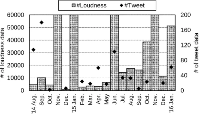
All of the collected data are shown in Figure 6 as a histogram of the number of data. Huge numbers of data were recorded in November 2014, January 2015, June 2015 and November 2015. As a result of the data collection experiments described in Section 4, the number of data in November 2014 and Jan-uary 2015 is substantial. We published the recording applica-tion in June 24, 2015, and consequently, the number of data in
0 40 80 120 160 200 0 10000 20000 30000 40000 50000 60000 '14 A ug . Se p. O ct . N ov. D ec. '15
Jan. Feb. Mar. Apr. May Jun
. Jul . Au g. Se p. O ct . N ov. D ec. '16 Jan. # o f tw e e t d a ta # o f lou d n e ss d a ta #Loudness #Tweet
Fig. 6: Number of collected data
June 2015 is also large. We conducted a recording experiment with our application from November 28, 2015 to November 29, 2015, resulting in a large number of data in November 2015 as well.
6. CONCLUSION
In this paper, we developed a client-server application for col-lecting environmental sounds using smart devices, and we used the developed application to conduct a sound collection experiment with 14 participants. The collected data were an-alyzed for the distribution of loudness levels and sound types. In particular, we can find an effect of the opening of a large shopping mall in the city from time series charts. Finally, we attempted to collect sound data using crowdsourcing.
The effectiveness of the system has been demonstrated through the experiments, but there remains future work to be done. For example, the microphone specification must be appropriately calibrated, if it is to be used for more users. The calibration parameters of an unknown device might be estimated from the parameters of known devices and a small amount of data recorded by the unknown device.
7. REFERENCES
[1] M. Matsuoka, N. Ueda, H. Tokuda, R. Lea, and L. Mu˜noz, “SmartCities15: International workshop on smart cities: People, technology and data,” in Pro-ceedings of UbiComp/ISWC15 Adjunct, Sept. 2015, pp. 1509–1513.
[2] D. Gooch, A. Wolff, G. Korteum, and R. Brown, “Reimagining the role of citizens in smart city projects,” in Proceedings of UbiComp/ISWC15 Adjunct, Sept. 2015, pp. 1587–1594.
[3] N. D. Lane, E. Miluzzo, H. Lu, D. Peebles, T. Choud-hury, and A. T. Campbell, “A survey of mobile phone sensing,” IEEE Communications Magazine, vol. 48, no. 9, pp. 140–150, Sept. 2010.
[4] W. Z. Khan, Y. Xiang, M. Y Aalsalem, and Q. Arshad, “Mobile phone sensing systems: A survey,” IEEE Com-munications Surveys and Tutorials, vol. 15, no. 1, pp. 402–407, Feb. 2013.
[5] S. Hara, M. Abe, and N. Sonehara, “Sound collec-tion and visualizacollec-tion system enabled participatory and opportunistic sensing approaches,” in Proceedings of CASPer-2015, Mar. 2015, pp. 390–395.
[6] J. Burke, D. Estrin, M. Hansen, A. Parker, N. Ra-manathan, S. Reddy, and M. B. Srivastava, “Partici-patory sensing,” in Proceedings of ACM workshop of World-Sensor-Web, Oct. 2006, ACM Sensys, pp. 117– 134.
[7] J. Goldman, K. Shilton, J. A. Burke, D. Estrin, M. Hansen, N. Ramanathan, S. Reddy, V. Samanta, M. Srivastava, and R. West, “Participatory sensing: A citizen-powered approach to illuminating the patterns that shape our world,” Woodrow Wilson International Center for Scholars, Washington, D.C., May 2009. [8] A. T. Campbell, S. B. Eisenman, N. D. Lane,
E. Miluzzo, and R. A. Peterson, “People-centric urban sensing,” in Proceedings of WICON-06, Aug. 2006, Ar-ticle No. 18.
[9] R. Rana, C. Chou, S. Kanhere, N. Bulusu, and W. Hu, “Ear-Phone: An end-to-end participatory urban noise mapping system,” in Proceedings of IPSN-2010, Apr. 2010, pp. 105–116.
[10] E. D’Hondt, M. A. Stevens, and A. Jacobs, “Partici-patory noise mapping works! an evaluation of partici-patory sensing as an alternative to standard techniques for environmental monitoring,” Pervasive and Mobile Computing, vol. 9, no. 5, pp. 681–694, Oct. 2013. [11] I. McGraw, C.-y. Lee, L. Hetherington, S. Seneff, and
J. R. Glass, “Collecting voices from the cloud,” in Pro-ceedings of LREC 2010, May 2010, pp. 1576–1583. [12] M. Matsuyama, R. Nisimura, H. Kawahara, J. Yamada,
and T. Irino, “Development of a mobile application for crowdsourcing the data collection of environmen-tal sounds,” in Human Interface and the Management of Information. Information and Knowledge Design and Evaluation, S. Yamamoto, Ed., vol. 8521, pp. 514–524. Springer, 2014.
[13] C. A. Kardous and P. B. Shaw, “Evaluation of smart-phone sound measurement applications,” Journal of Acoustical Society of America Express Letters, vol. 135, no. 4, pp. EL186–192, Apr. 2014.
[14] H. Fletcher and W. A. Munson, “Loudness, its defini-tion, measurement and calculadefini-tion,” Journal of Acousti-cal Society of America, vol. 5, no. 82, pp. 82–108, Oct. 1933.