Tech Bull Fac Agr Kagawa Univ
,
Vol 37, No 2, 131- 148, 1986STUDIES ON THE ASSESSMENT OF THE ALLOWABLE STOCKING
CAPACITY OF YELLOWTAIL CULTURED
IN THE FUKAURA FISH FARM
(11)
Numerical investigations on tidal current
Takashi SASAKI,
Teekawuth
POTAPIROM"
and Hiroo
INOUE
A series of researches have been undertaken on assessments of stocking capacity of a marine culture farm in Fukaura- wan located in Wakamatsu-seto, Nagasaki-ken The present paper reports on a part of these researches, and its purpose is to prepare the field of tidal currents in a fonn suitable for subsequent water quality analysis and ecological simulation
For that reason, numerical calculation of tidal currents around Wakamatsu-set0 including Fukaura-wan was car- ried out, from the macroscopic stadpoint The reliability of the numerical analogy was examined by means of com- parisons between actual observations and computed results
Consequently, it was shown that the numerical results were in good agreement with the observed data,
Introduction
We have undertaken researches on assessments of stocking capacity of a marine culture farm in Fukaura-wan lo- cated in Wakamatsu-seto, Nagasaki-ken The present paper reports on a part of these researches, and its purpose is to clarify the feature of the tidal currents in a form suitable for subsequent water quality analysis and ecological simulation. The tidal currents in and out of the basin were numerically investigated As a numerical technique, a finite-difference method derived by Ueno has been
Numerical calculation of the tidal currents was proceeded under limitation of our computer as follows: First, the computations of the tidal currents were practiced on a rough g ~ i d model, referred to in this paper as MODEL I The computed area of Wakamatsu-set0 including Fukaura-wan is 6.0 km long (N-S direction) and 4 2 km wide (E-W direc- tion) The grid point interval is 100 m and time step is 6 0 sec The variations in sea level as the boundary conditions were given a t each outside of two mouthes of Wakamatsu-set0
Next, in order to understand sea water flows in and near Fukam-wan in detail, the computations of the tidal currents were practiced on a fine grid model located within the rough grid model, referred to in this paper as MODEL I1 The computed * Kasetsart University, Bangkok in Thailand
132 Tech Bull Fac Agr Kagawa Univ
,
Vol. 37, No 2 (1986)area is 2 6 km long (N-S direction) and 1 6 km (E-W direction) The grid point interval is 50 m and time step is 3 0 sec The sea level variations on both boundaries of the area were those obtained by computations on the rough grid model. This is the report about the numerical investigations on the tidal currents in Wakamatsu-seto, solved in the MODEL I
Method Theoretical considerations for hydrodynamic model (1),(2),(3),(4)
Coordinate system
The horizontal coordinate x is taken east-westward, and the other one y is taken north-southward The vertical coordinate
z
is downward The positive x is to the westward, while the positive y is to the southward The plane of x = 0 is considered to coincide with mean sea level.Definition
of
turbulenceThe flow is considered turbulent if the viscous forces are small relative to the inertial forces The water particles move in irregular paths which are neither smooth nor fixed The velocity of the particle and the pressure a t any point show random variations with time and space.
For any point, we may, according to Reynolds's procedure, set
where u, v, w and p are the momentary values of the velocity components corresponding to x, y and x directions, respectively and pressure Overscores and symbols of prime denote the time averaging values and the fluctuations of the values, respectively
The time average for u a t a fixed point in space is
where t is the time a t the mid point of the averaging period and T the interval time Definitjon of discharge
T i and F c a n be defined as follows
where U and V are vertically averaged velocities with respect to
x
and y, respectively. u, and v, are the devia- tions of the velocities with respect to x and y, respectively h is the elevation of the bottom with respect to mean sea level and 3. the elevation of water surface with respect to mean sea level.From Eq (3), the vertically averaged velocities are
The discharges are defined as follows
Takashi SASAKI, Teekawuth POTAPIROM and Hiroo INOUE: Allowable stocking capacity 133 Boundary conditions
In this model, three boundaries are to be treated; namely, bottom, sea surface and open boundary The condi- tions of the open boundaries are mentioned in the later
At the bottom we can put h(x, y ) - z = 0 Accordingly, we get
dh dh
~ b - f ~ b - - wb=O .
...
(6)dx dy
where ub, vb, and
w b
are velocities components a t the bottom ins
y, and z, respectively At the free surface we can put{(x,
y,t )
+
z = 0 and then, we getwhere us, vs and w, are the velocity components a t the free surface in
x,
y, and z, respectively ThereforeEquation of continu~ty
The equation of continuity in laminar flow is written as follows
where q is the specific density, V the velocity vector and
6
the Eulerian operatorThe continuity equation for an incompressible fluid with q = constant is obtained as follows.
div
V=OBy using the time averaging velocity, the continuity equation in turbulent flow is rewritten a s follows
3.27 d C 0
ax
aya~
(11)Integrating Eq (11) to obtain the horizontal two dimensional equation averaged vertically, we find
L h B d z + cdx lh*d2+ - r a y wb wS=O (12) From Eq (5), we obtain ah
a g
GdZzUb-+us-+ [ : g d 2 dx a x .a~ a
ahac
= - /
a yay.-,
f i d z = u b - + v s - + 1 X d z JY a y134 Tech Bull Fac Agr Kagawa Univ
,
Vol. 37, No. 2 (1986) Substituting E q (8) and Eq (13) into Eq (12), we obtainEquatlon of momentum
If the Coriolis force due to the influence of rotation of the earth is taken into consideration, the general form of Navier-Stokes equations can be written as follows
where V represents the velocity of fields in the xyz system and the components are (u, v and w )
w the earth's rotation angular velocity and the components are (a,, w y , w,),
K the external force per unit volume and the components are (O,O,g), where g is the gravitational acceleration, P the pressure a t any point (x,y,z),
Q the sea water density and v the coefficient of kinematic viscosity
From Eq (10) and Eq (15), Navier-Stokes equations for an incompressible flow can be reduced to
d V
at+
Vgrad V + 2 o x V = - g + v B V (16)For simplicity, the Coriolis force may be left out in the following considerations, since it is not a t this point essen- tial in the derivation of the stresses Thus Eq (16) can be written
(17)
where p is the coefficient of viscosity,
v=&
PThe above equations may be averaged over a sufficiently long time interval, a s in
d t
By using Eq. (1) and taking Q' = 0, Eq (17) for turbulent flow may be written as follows
d u d u - d a - d u
-+
zi-+ v-+w-
d t d x d y d z1
80 aii - 8 0 -aii-+
ZZ-+ v-+w-
d t d x d y d z P d y P (18)Takashi SASAKI, Teekawuth POTAPIROM and Hiroo INOUE: Allowable stocking capacity 135
Following the Prandtl's hypothesis, let consider for simplicity only the average flow, u , in the direction of z-axis to derive the relationship between stresses and average velocity Thus, from Eq. (I), we get
Similarly, taking only the average flow in the direction of y-and z-axis, we can put
And the stresses in Eq (18) can be expressed by
where
l x x l Y X I,, ZXY I Y Y l z y
1 x 2 ZY2 12.2
I !
136 Tech. Bull Fac Agr Kagawa Univ., Vol. 37, No 2 (1986)
are the eddy viscosity coefficients
If Eq (21) is substituted into Eq (18), the hydrodynamic equations for the average velocities in turbulent flow, with the coriolis force, can be written
(
dii@=
~t - & 9 + 2 , p a x sin - ( A ~ ~ + P ) ~ ) P dxaa
Do
- --- do --!
G + 2 w sin + ' [ A ( ( A ~ ~ + ~ & ) D t P dy P dx (22) -- I[ a (
dw D w - - & ~ - s - ~ w c ~ s ~t paz
*a+:
-
( A ~ , + L ~ ~ ) Pax
a
d dw + a ( ( ~ z y+
P&) + z ( ( ~ - + P)z))where $ is the geographical latitude of a place, and
When ocean currents are dealt with, it seems that only shearing stresses resulting from horizontal velocity com- ponents (C and
F)
are of importance The vertical velocity components a s well as its gradients are usually small enough to be neglected in the equations of motion and so is the coefficient of viscosity is similarAnd then, following the assumptions that the coefficients of vertical (A,) and horizontal (A1) eddy viscosity are constant in the ocean are accepted, Eq (22) may be rewritten
D t (23)
-- -
Do-
2w sin *G-T-+T 1 d P A L d2ii d2ii-+-
+-=
A d20 -D t p a ,
,(ax2
dy2) A d z 2 ) (24)1 dP
o=-_--g
P 3.2 (25)
where f i = ~ g ( z +
c)
Takashi SASAKI, Teekawuth POTAPIROM and Hiroo INOUE: Allowable stocking capacity 137
where f = 2 0 sin $
We shall first define the terms on the left hand side and then the terms on the right hand side respectively Using Eq (5), We obtain
ah
in which
-=O.
at
In Eq (26), convective terms on the left hand side are transformed
Substituting Eq (11) into Eq (29) and integrating with respect to z yields
in which
From Eq (30) and Eq (31), then we obtain
138 Tech Bull. Fac Agr. Kagawa Univ., Vol 37, No. 2 (1986) Similarly, in the y direction, we also obtain
In right hand sides of Eq (26) and Eq (27), the tangential stresses a t the sea surface and the bottom are usually denoted by rs and 7b respectively Hereunder, the wind effects may be neglected
h A a2a A dii A, dii
.Li
;
d z 2 ) d ~ = l $ z l k - 1 7 z l ~in which
From theoretical considerations, it is found that the bottom stress can be expressed by a term of the form
where C is the Ch6zy coefficient
In oceanographic studies, for convenient use, this relation is written as
where y2 is a non-dimensional constant and is related to C by
The values of C and y2 depend on the roughness of the bottom which is a function of the depth and the bottom material Therefore in case of a shallow sea, it is necessary to determine the value of y2.
According to Rossby and Bowden, the value of r2 in the sea had been found to be
An analogous effect is found in the Manning's formula We will describe it in a following paper Then, Eq (35) reduce to
Takashi SASAKI, Teekawuth POTAPIROM and Hiroo INOUE: Allowable stocking capacity 139 As for the last terms of Eq (26) and Eq (27), the values are too small t o be considered with the all of them Because of all of them are determined with time step At But these terms are necessary to smooth the flow, so these terms will be computed seperately with AT
Here, At is the time step which corresponds to wave propagation and AT is the time step for output
where
W A K A M A T S U - S E T
BOUNDARY L O C A T I O N N AND S E L E C T E D S T A T I O N 0 0 0.2 0.9 0.6 0.8 1.0 DIBTANCE BCRLEtKHFig 1 Analysis-area for the finite-difference method with square meshes; RA-RT: monitoring stations of tidal elevation, QA -QT: monitoring stations of tidal current, I
-
L: boundary locationBy substituting Eq (33) and Eq (40) into Eq (26), the Navier-Stokes equation in the x direction is written
140 Tech. Bull. Fac Agr Kagawa Univ., Vol. 37, No 2 (1986) Similarly, in the y direction, we obtain
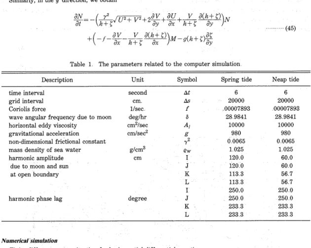
Table 1 The parameters related to the computer simulation
Description Unit Symbol Spring tide Neap tide
time interval grid interval Coriolis force
wave angular frequency due to moon horizontal eddy viscosity
gravitational acceleration
non-dimensional frictional constant mass density of sea water harmonic amplitude
due t o moon and sun a t open boundary
harmonic phase lag
second cm llsec deglhr cm2/sec cm/sec2 degree Numerical simulation
Finite-difference approximation for basic partial dzfferentza equations
The equations of motion, Eq (44) and Eq (45), and the equation of continuity, Eq (14), may be transformed into the following finite-difference equations(1)p(2) in order to obtain the discharges X in the x-direction and Y in the y-direction, and the fluctuation from the mean sea level, 5
Takashi SASAKI, Teekawuth POTAPIROM and Hiroo INOUE: Allowable stocking capacity 141
By using the discharges (X, Y) obtained from Eqs (46) and (47), the tidal currents (U, V) are given by
E q (42) and Eq (43) can be expressed by the following finite-difference equations
where As is the grid interval, At the time step, A T the time step larger than A t , (%,j) the discrete point to calculate the tidal levels and (1,m) the discrete point to calculate the tidal currents
Boundary conditions and inltial cond~tions
The components of the velocity perpendicular to the coast must be zero along the coast but the tides or currents in the open boundaries must be ascertained Therefore, the boundary conditions can be written as follows
where GO,? is the mean amplitude of the consituent, taken as ( M 2 + S z ) a t spring tide and ( M z - S 2 ) a t neap tide,
Tech Bull Fac Agr Kagawa Univ
,
Vol. 37, No. 2 (1986) +20 CM/SEC --- , - - . ]-T=L-- -- CYCLE 2 NO h h CYCLE 3 RD E Q -1 LI ++ CYCLE 2 KD U CYCLE 3 RD -20 1 2 3 4 5 6 7 8 9 10 1 1 12 13 T I H E I H RFig 2 Changes in tidal current with time over three tide cycles; QD(21,37), spring tide
With regards to initial conditions, the tidal levels and currents a t the starting time of caculation are taken to be zero over the entire area; that is
5t4,=0, X t m = Ytm=O (51)
Stability and convergence
The stability and convergence conditions for explicit scheme are related to the propagation velocity of a long wave in the sea In practice, it is usually assumed as follows
where As is the size of the grid, At the time-step, h,, the maximum depth in the sea area and g the acceleration due to gravity
Takashi SASAKI, Teekawuth POTAPIROM and Hiroo INOUE: Allowable stocking capacity 143 Results and discussion
The finite-difference equations of motion and of continuity for tidal dynamics, Eqs (46),(47) and (48), could be numerically solved on the grid of MODEL I shown in Fig 1, under the initial and boundary conditions given by Eqs (50) and (51) The computed area including Fukaura-wan was 6 0 km long (N-S direction) and 4 2 km wide (E-W direction) The size of the square grid was 100 x 100m2 The north and south boundaries were located on the latitude 32'54' N and 32'51' N respectively The variations in sea level were given as the boundary conditions on each outside of two mouthes Variations in the tidal level and current a t the starting time of caluculation were taken to be zero over the computed area, according to E q (51). The parameters related to the computation are summa- rized in Table 1
In this case, acceptable mesh sizes in space and time, namely As12 and At, were estimated to be 100 m and 6 sec, respectively, according to the stability criteria shown as Eq (52) Fig 2 shows an example of test on stability and convergence for the present numerical analysis In the figure, results of tidal currents obtained a t a monitoring station, QQ (z = 2 1 , j =29), in Wakamatsu-set0 are illustrated for three tidal cycles Fig 2 indicates that the conver- gence and the stability of the numerical analogy for the hydrodynamic model were very well
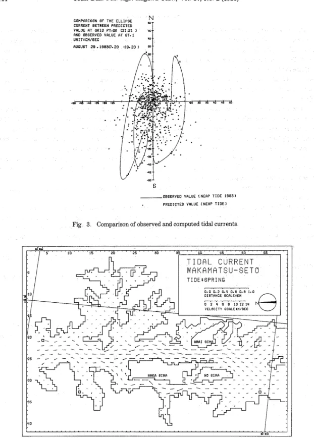
Fig 3 shows the computed values of tidal currents a t a monitoring station, QK (2 =22,7 =22), during neap tide Actual measured currents(5), obtained on August 29, 1983, were superimposed on this figure and good agreement was seen between the computed and measured currents
The tidal currents computed a t other various points were also checked to get the reliabilty of the present numeri- cal analogy
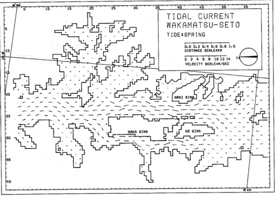
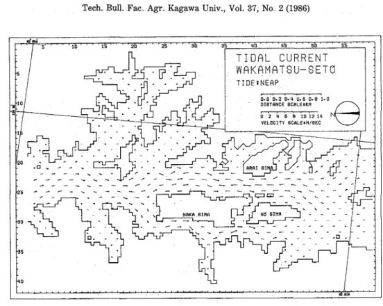
The distributions of tidal currents in Wakamatsu-set0 are shown in Figs 4-5 Fig 4 shows tidal currents 2 hrs before spring high tide Fig 5 shows tidal currents a t the same time before neap high tide The tidal currents in Wakamatsu-set0 are extremely fast However, the tidal currents in Fukaura-wan are weak enough to permit the fish faming Fig 6 shows the Tidal residual flow a t neap tide From this figure, it is found that many circulation flows caused by the complicated topography were formed in front of the bay mouth and behind the island
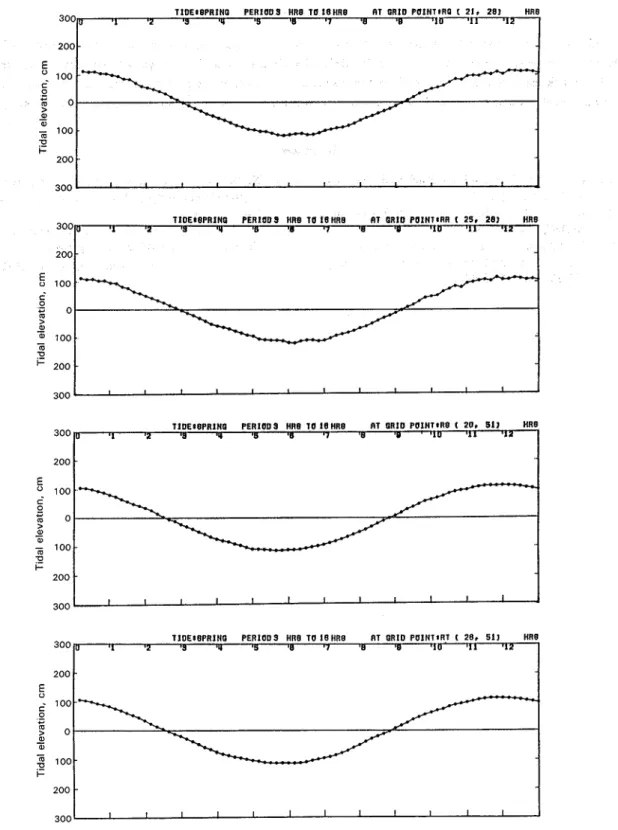
The tide curves during the spring tide calculated a t the four monitoring stations, RQ(2 =21,1=28), RR(25,28), RS(20,51) and RT(26,51) in Fig I , are shown in Fig 7
The present computed results are kept on a magnetic tape and those will be used a s the boundary conditions and initial conditions for MODEL I1 treated in a following paper
Concluding remarks
In the first repord5), the tidal current data observed in and out of Fukaura-wan were analysed and we made the following findings The largest values of observed tidal currents a t Stn 1 (the main stream) were about 70 1 cmlsec (westward flow) in the E-W component and about 133 1 cmlsecc (northward flow) in the N-S component Those values a t Stn 2 (the mouth of Fukaura-wan) were 14 6 cmlsec (eastward flow) and 61 7 cmlsec (southward flow) The N-S component flow was predominant a t both Stn 1 and Stn 2. The E-W component flow was extremly small The northward currents were larger than the southward currents a t both stations I t seems to be an asymemetrical flow because both of them are complicated by topography
In this report, numerical experiments were carried out on the basis of those current data I t was shown that the observed tidal currents were in agreement with the predicted values based on a two-dimensional numerical model, MODEL I We confirm that the computed results obtained are those to be used sufficiently
144 Tech. Bull. Fac Agr. Kagawa Univ
,
Vol 37, No 2 (1986)N
COMPRRISON OF THE ELLIPSE ---
CURRENT BETREEN PREDICTED w T
VRLUE RT GRID PT-OK ( 2 1 2 1 I
RND OBSERVED VRLUE AT 61.1
UNITZCM/GEC
1
RUGUST 2 9 ,19830.20 1 9 - 2 0 1
st
O B S E R V E D VRLUE CNERP TIDE 19831
PREDICTED VRLUE (NERP TIDE 1
Fig 3 Comparison of observed and computed tidal currents
dn; 5' ' ' ' ' l b ' ' " 1 5 ' ' ' ' 2 b 2 5 ' " ' s b ' " ' 3$ " - " s b , , ' " A ' " , sb" " 5 5 " " .
T I D A L
C U R R E N T
W A K A M A T S U - S E T 0
. ,< .? -. .- ... .- .- .-.-
. . . . . . . . ^-
. . .
. . . ., .. ,, . 3 5 '40 P 8'"Takashi SASAKI, Teekawuth POTAPIROM and Hiroo INOUE: Allowable stocking capacity 145 . da; 5' " ' . l b 25 ' ' ' '3b ' 3 8 ' " '4b 4 5 ' " '5b 58 '
T I D A L C U R R E N T
sW A K A M A T S U - S E T 0
T I D E l S P R I N G 0.0 0.2 0.4 0.6 0-8 1.0 OISTRNCE SCRLEtKM V E L O C I T Y S C R L E l M l S E C ..a -....
4.. .
-
-. -. " R R R I S I M ,-. -. &. -. -. . . \. -. -....
,
,
., -. - , - . - . . . . -. . . . . .. .iI,"Fig. 4-b. Distribution of maximum tidal stream during ebb tide a t spring tide
Tech. Bull. Fac Agr. Kagawa Univ., Vol. 37, No 2 (1986)
Fig 5-b. Distribution of maximum tidal stream during ebb tide a t neap tide
Takashi SASAKI, Teekawuth POTAPIROM and Hiroo INOUE: Allowable stocking capacity 147
300 I 2 TIDEt8PRlNQ 3 Y PERIODS HR8 T O l 8 H R 8 4 B 7 8 AT ORID POINTtRP B C 21, 2 8 1
3007) 1 2 TIOE*BPRINP 3 1 PERIODS HR8 TO18HR8 6 a 7 8 AT PRID POlNTtRR 0 1 0 ( 25, 2 8 1 '11 '12 HA8
200 -
5
1 0 0 . ig
0 .5
-
1 0 0 ,-
m P + 200 .TIDE*8PRINQ PERIODS HR8 TO 1BHR8 RT ORID PUINT*RT ( 28, 5 1 1
200 3 0 0 1 - as ~8 ~7 t8
Tdl
300 7 ) TIDEI8PRINQ PERIODS HRB 1 0 18HR8 AT QRlD POlNTtR8 ( 2 0 1 5 1 1 HA8
Fig. 7 Changes in tidal elevations with time in the monitoring station; RQ(21,28), RR(25,28), RB(20,51) and RT(28,51); spring tide
200
1 2 8 Y 6 B 7 8 0 "10 '11 '12
148 Tech Bull Fac Agr Kagawa Univ
,
Vol 37, No 2 (1986) AcknowledgmentsThis work was supported by the Nagasaki Fishery Experimental Station, Nagasaki-ken The data analysis in the present paper was carried out on a MELCOM-COSMO-700s in the data station of Kagawa University The authors wish to thank the scientists and the staffs of these stations for helping in the field surveys and the data analysis The authors also would like
to
thank Mr Yoshihiko Tsuruta, a graduate student, for his cooperation in this studyReferences
( 1 ) UENO T: Bull of the Kobe Marine Observatory, ( 4 ) NUEMANN G and PIERSON W J: Principles of
No 179, 1-116 (1967) Physical Oceanography, N J
,
Prentice-Hall, Inc,
( 2 ) UENO T: Bull of the Kobe Marine Observatory, 184-190 (1966)No 187, 1-88 (1971) ( 5 ) SASAKI. T and INOUE H: Tech Bull Fac Agr ( 3 ) DRONKERS J J: Tidal computations, Amster- Kagawa Univ Vol37, No 1 (in press)
rdam, Nor thholland Publishing Company, (Received October 31, 1985) 177-255, 372-405 (1964)