ALGEBRAIC ALGORITHMS FOR D-MODULES AND NUMERICAL ANALYSIS
TOSHINORI OAKU, YOSHINAO SHIRAKI, and NOBUKI TAKAYAMA Department of Mathematics, Tokyo Women’s Christian University, Speech and
Motor Control Res. Group, NTT Communication Science Labs., and Department of Mathematics, Kobe University.
Algorithmic methods in D modules have been used in mathematical study of hy-pergeometric functions and in computational algebraic geometry. In this paper, we show that these algorithms give correct algorithms to perform several operations for holonomic functions and also generates substantial information for numerical evaluation of holonomic functions.
1. Introduction
As was observed by Castro and Galligo [3] , [5], the Buchberger algorithm for computing Gr¨obner bases of ideals of the polynomial ring applies also to the Weyl algebra, i.e., the ring of differential operators with polynomial coefficients. This generalization of the Buchberger algorithm has turned out to be very fruitful in the computational approach to the theory of D-modules, which aims at an algebraic treatment of systems of linear partial (or ordinary) differential equations and the theoretical foundation of which was laid by Bernstein, Kashiwara, M. Sato, and many others.
The aim of this paper is to show that such an algorithmic approach to the D-module theory, which essentially depends on the Buchberger algo-rithm, enables us to solve some fundamental problems in symbolic compu-tation, namely to perform computation with so-called holonomic functions. Our motivation of studying computation with holonomic functions comes from signal processing and numerical analysis. We sketch some applications of computation of holonomic functions to these areas.
A function u is called holonomic, roughly speaking, if u satisfies a sys-tem of linear differential equations P1u = . . . = Pru = 0 whose solutions
form a finite dimensional vector space; here P1, . . . , Prare elements of the
Weyl algebra Dn = Chx1, . . . , xn, ∂1, . . . , ∂ni over the field of the complex
numbers with ∂i= ∂xi=
∂
∂xi. Such a system is called holonomic and plays
a key role in the theory of D-modules.
Since a linear ordinary differential equation is always holonomic, special functions of one variable, such as the Gauss hypergeometric function and the Bessel function are holonomic by definition. Moreover, the rational functions of arbitrary number of variables and their exponentials are simple examples of holonomic functions. As nontrivial examples, the expression fλ for an arbitrary polynomial f and an arbitrary complex number λ and
GKZ-hypergeometric systems (see, e.g., [18]) are holonomic.
We can expect to obtain substantial information on a holonomic func-tion by studying the differential equafunc-tions which it satisfies, rather than dealing with the function itself. This holonomic approach to special func-tion identities was initiated by Zeilberger et al. ([1], [22], [16], [23]).
We are concerned with the following computational issues on holonomic functions: (1) Given two holonomic functions f , g and two differential operators P , Q, find a holonomic system which the function P f + Qg satisfies; (2) Given two holonomic functions f , g, find a holonomic system which the function f g satisfies; (3) Given a holonomic function f (t, x), find a holonomic system which the integralRCf (t, x) dt satisfies.
We give answers to the three problems (under a technical condition for the third one) by using the Buchberger algorithm applied to the Weyl algebra. The class of holonomic functions are stable under these three operations (addition, multiplication, integration) and two more operations of restriction and localization [13]. We give explicit algorithms for these constructions. Partial answers to the above three problems were given in [1], [19], [22], [23].
2. Holonomic functions
Definition 2.1. A multi-valued analytic function f defined on (the univer-sal covering of) Cn\ S with an algebraic set S of Cn is called a holonomic
function if there exists a left ideal I of Dnso that M = Dn/I is a holonomic
system and P f = 0 holds on Cn\ S for any P ∈ I.
We set Ann(f ) := {P ∈ Dn| P f = 0 on Cn\ S}. Then f is holonomic
if and only if Dn/Ann(f ) is holonomic.
Proposition 2.2. [2] Let f ∈ C[x] be a nonzero polynomial and let λ be an arbitrary complex number. Then fλ is holonomic.
Algorithms to compute a holonomic system which fλ satisfies are given
Proposition 2.3. Let f and g be holonomic functions and P, Q ∈ Dn. Then P f + Qg and f g are holonomic.
We shall give an algorithmic proof to this proposition in Section 3.3. The class of the holonomic functions is not closed under the division [23]. Proposition 2.4. Let f ∈ C(x) be a rational function. Then f , exp(f ), and log f are holonomic.
Proof. Suppose f = p/q with p, q ∈ C[x]. Then by Proposition 2.2, p and q−1 are holonomic. Hence f is holonomic by Proposition 2.3. The
holonomicity of exp(f ) is a special case of the proposition below. To prove that u := log f is holonomic, we may assume that f is a polynomial. Then u satisfies f ∂if = fi with fi := ∂i(f ). Let fi be of degree ni with respect
to xi. Then we have ∂inif ∂iu = 0 (i = 1, . . . , n). Then, this system is
identified with the left Dn-module M = Dn/(DnP1+ . . . + DnPn) with Pi := ∂inif ∂i and M is a holonomic system on {x ∈ Cn | f (x) 6= 0} since
Char(M ) ⊂ {(x, ξ) | ξif (x) = 0 (i = 1, . . . , n)}. In view of Theorem 3.1
of Kashiwara [7], the localization M [1/f ] is holonomic. Since M [1/f ] is isomorphic to M outside f = 0, we are done.
We note that an algorithmic method for the localization is given in [13]. Proposition 2.5. [1] Let f be a multi-valued analytic function and assume that (∂f /∂xi)/f is a rational function for every i = 1, . . . , n. Then f is holonomic.
Proof. Put ai := (∂f /∂xi)/f = pi/qi with pi, qi ∈ C[x]. Then f satisfies M : (qi∂i− pi)f = 0 (i = 1, . . . , n). Let q be the least common
mul-tiple of q1, . . . , qn. Then M is holonomic outside the hypersurface defined
by q = 0. This implies that f is holonomic in the same way as the proof of the preceding proposition.
Example 2.6. For two polynomials f1(x), f2(x) in C[x1, . . . , xn], put f (x) = exp(f1(x)/f2(x)). The system of differential equations M above
is not holonomic in general (consider, e.g., exp(1/(x3
1− x22x23))). A
holo-nomic system for f (x) can be found by the method in [13].
Let f be a holonomic function. By definition, it is a multi-valued an-alytic function defined on Cn\ S. The algebraic set S is contained in the
zero set of ¡in(0,1)(I) : (ξ1, . . . , ξn)∞
¢
∩ C[x1, . . . , xn], generators of which
are computable by the Buchberger algorithm in D from generators of I. See [9] and [18, §1.4].
3. Four operations on holonomic functions 3.1. Restriction to xm+1 = · · · = xn = 0
Let u(x) be a holonomic function and suppose that a left ideal I of Dn
is explicitly given so that M := Dn/I is a holonomic system. Then MY = M/xnM is a holonomic system. This holonomic system is called
the restriction of M to xn = 0. As a left Dn−1-module, MY is
gener-ated by the residue classes of 1, ∂n, . . . , ∂nk0. Hence, there exists a
sub-module J such that Dk0+1
n−1 /J ' MY; J is a system of equations for u(x0, 0), (∂
nu)(x0, 0), . . . , (∂nk0u)(x0, 0), where x0 = (x1, . . . , xn−1). An
al-gorithm of finding generators of J from those of I is given in [11]. By an elimination, we can find a system of equations for u(x0, 0) from J [18, §5.2].
Take an integer m such that 0 ≤ m < n. Let Z be the algebraic set {(x1, . . . , xn) | xm+1 = · · · = xn = 0} and M a left Dn-module Dnr/I
where I is a left submodule of Dr
n. The restriction of M to Z is defined by M/(xm+1M +· · ·+xnM ) and is denoted by MZas in the case of the
restric-tion to a hypersurface. It follows from the definirestric-tion we have M/(xn−1M + xnM ) ' ((M/xnM )/xn−1(M/xnM )), M/(xn−2M + xn−1M + xnM ) '
(((M/xnM )/xn−1(M/xnM )) xn−2((M/xnM )/xn−1(M/xnM ))) and so
on. Therefore, the iterative application of the restriction algorithm for the hypersurface case provides an algorithm to get the restriction MZ. Yet
another algorithm which computes the restriction MZ without the iteration
is given in [18, §5.5], which uses weight vectors. It is an interesting question to compare the two methods from the efficiency point of view. We finally note that the book [18] and our discussion consider restrictions of a singly generated left D-module D/I, but it is straightforward to generalize it in the case of Dm/I.
3.2. Integrals of holonomic functions with parameters
Let f (x) be a holonomic function and let I be a left ideal of Dn such
that M := Dn/I is a holonomic system and I ⊂ Ann(f ). For the sake
of simplicity, let us assume that f (x) is infinitely differentiable on Rn
and rapidly decreasing with respect to xn, i.e., limxn→∞x
j
n∂nkf (x) = 0
holds for any x0 := (x
R∞
−∞xknf (x0, t) dt (k ∈ N). Then g0(x0), g1(x0), . . . , gk0(x
0) are solutions
of the holonomic system M/∂nM where k0 is the maximal non-negative
integral root of the associated b-function (see also [1],[19] although only g0
is considered there). Computation of M/∂nM can be reduced to that of M/xnM by an isomorphism of Dn induced by the Fourier transform. See,
e.g., [18, §5.5] for details.
3.3. Sum and product of holonomic functions
Let u be a holonomic function and suppose that a left ideal I of Dn is
given so that I ⊂ Ann(u) and M := Dn/I is holonomic. First, for a given Q ∈ Dn, we show that we can compute a holonomic system for Qu. The
fact that Qu is holonomic follows from DnQu ⊂ Dnu. Let P1, . . . , Pr be
generators of I. Then for P ∈ Dn, P Q ∈ I holds if and only if there exist Q1, . . . , Qr ∈ Dn such that P Q + Q1P1+ . . . + QrPr = 0. By computing
a Gr¨obner basis of the ideal generated by Q, P1, . . . , Pr, we can obtain
generators of their syzygy module
S := {(P, Q1, . . . , Qr) ∈ Dr+1n | P Q + Q1P1+ . . . + QrPr= 0}.
Then the projections of generators of S to the first component generate the left ideal I : Q = {P ∈ Dn | P Q ∈ I}. Thus we have I : Q ⊂ Ann(Qu).
The left Dn-homomorphism Dn3 P 7→ P Q ∈ Dn induces a homomorhism Dn/(I : Q) → Dn/I, which is injective by the definition of I : Q. Hence Dn/(I : Q) is holonomic.
Now let v be another holonomic function with an explicitly given left ideal J ⊂ Ann(v) so that Dn/J is a holonomic system. Our first aim is to
compute a holonomic system for P u + Qv for given P, Q ∈ Dn. Since the
holonomic systems for I : P and J : Q are computed in the way described above, we may assume that P = Q = 1. Then we have I ∩ J ⊂ Ann(u + v). This ideal intersection can be computed by the Buchberger algorithm in the same way as in the polynomial ring (see, e.g., [4]). Dn/(I ∩ J) is
a holonomic system since the homomorphism Dn 3 P 7→ (P, P ) ∈ D2n
induces an injective homomorphism Dn/(I ∩ J) −→ (Dn/I)
M
(Dn/J).
Next let us consider an algorithm to find a holonomic system for the product uv. Let Gu and Gv be finite sets of generators of I and J respectively. Put D2n = C[x, y]h∂x, ∂yi with y = (y1, . . . , yn) and ∂x:= (∂x1, . . . , ∂xn), ∂y := (∂y1, . . . , ∂yn). Let Iu⊗v be a left ideal of D2n
generated by both Gu(x) := {P (x, ∂x) | P ∈ Gu} and Gu(y) := {P (y, ∂y) | P ∈ Gv}. Then it is easy to see that Iu⊗v ⊂ Ann(u(x)v(y)) and that Mu⊗v := D2n/Iu⊗v is holonomic. Put ∆ := {(x, y) ∈ C2n | x = y}. Then
the restriction of M to ∆:
M∆:= D2n/((x1− y1)D2n+ · · · + (xn− yn)D2n+ Iu⊗v)
can be computed by performing coordinate transformation xi− yi → yi
and xi → xi and then applying the restriction algorithm with respect to
the variables y1, . . . , yn. Note that M∆ is holonomic since holonomicity is
preserved under restriction. In fact, M∆ is nothing but the tensor product
of Dn/I and Dn/J over C[x], and the above algorithm was introduced in
[12]. From M∆, we can compute a left ideal Iuv of Dn so that Dn/Iuv is a
holonomic system for u(x)v(x) by elimination.
The above algorithm for Iuv is for general purpose but is not efficient
since it involves restriction to the n-dimensional linear space in the 2n-dimensional space. Hence possible short cuts for some particular cases would be worth mentioning. As one of such cases, consider v := efu with
a holonomic function u and a polynomial f . Suppose given a left ideal I ⊂ Ann(u) such that Dn/I is holonomic. Put fi := ∂f /∂xi. Then the left
ideal J of Dn generated by
{P (x1, . . . , xn; ∂1− f1, . . . , ∂n− fn) | P (x1, . . . , xn; ∂1, . . . , ∂n) ∈ I}
is contained in Ann(v) since (∂i−fi)•(efu) = ef(∂i•u). The characteristic
variety of Dn/J is
{(x, ξ1− f1(x), . . . , ξn− fn(x)) ∈ C2n| (x, ξ) ∈ Char(Dn/I)}.
Hence Dn/J is holonomic. As another case, the product of a holonomic
function and the Heaviside function will be discussed later.
4. Holonomic distributions and their integrals
Since some important analytic holonomic functions are expressed as definite integrals of distributions, the notion of holonomic function should be gen-eralized; we will introduce holonomic distributions. They are closed under four operations if the result of an operation is well-defined. Computation of these operations can be done by the same algorithms as in the case of holonomic functions.
Definition 4.1. Let u be a distribution (in the sense of Schwartz) defined on Rn. Then u is said to be a holonomic distribution if there is a left ideal
I of Dn so that Dn/I is holonomic and P u = 0 holds as distribution for
any P ∈ I.
For example Dirac’s delta function δ(x) = δ(x1) · · · δ(xn) is a holonomic
distribution since x1δ(x) = · · · = xnδ(x) = 0. Let us introduce the
Heav-iside function Y (x1) defined by Y (x1) = 0 for x1 < 0 and Y (x1) = 1 for
x1 ≥ 0. Then we have ∂1Y (x1) = δ(x1) as distribution derivative. The
Heaviside function is a holonomic distribution since it satisfies the holo-nomic system x1∂1Y (x1) = ∂2Y (x1) = · · · = ∂nY (x1) = 0. As another
example of holonomic distribution, let f (x) be a polynomial with real co-efficients and λ be a complex numer. Then we introduce the symbol
f (x)λ +:=
½
f (x)λif f (x) ≥ 0
0 if f (x) < 0. It is easy to see that f (x)λ
+is well-defined as a tempered distribution if the
real part of λ is positive by the pairing hf (x)λ +, ψ(x)i = Z Rn f (x)λ +ψ(x) dx
for rapidly decreasing smooth functions ψ(x). By virtue of the identity of the Bernstein-Sato polynomial
P (λ)f (x)λ+1+ = bf(λ)f (x)λ+
with the Bernstein-Sato polynomial bf(s) ∈ C[s] of f (x) and some P (s) ∈ Dn[s], the tempered distribution f (x)λ+ can be analytically continued to
the whole complex plane as a meromorphic function with respect to the parameter λ. The possible poles are contained in the set
{r − ν | r ∈ C, bf(r) = 0, ν = 0, 1, 2, . . .}, (4.2)
which is in fact a subset of the negative rational numbers according to the celebrated theorem of Kashiwara [6]. Put Ann(fs) := {P (s) ∈ D
n[s] | P (s)fs= 0}. Then the algorithm in [10] produces a set G of generators of
Ann(fs). If λ does not belong to the exceptional set (4.2), then we have P (λ)f (x)λ
+= 0 for any P (s) ∈ G. This follows easily from the definition of
the action of P (s) on fsviewed as a multi-valued analytic function together
with analytic continuation. However, even if P ∈ Dn annihilates fλ as an
analytic function, it does not necessarily annihilates f (x)λ
+as a distribution.
For example, we have ∂x(1) = 0 but ∂x1+= ∂xY (x) = δ(x) 6= 0 with n = 1.
is holonomic [6, Prop 6.1]. Hence the distribution f (x)λ
+ is holonomic if λ
does not belong to (4.2).
The integral of a holonomic distribution with respect to some variables is again holonomic and can be computed by the integration algorithm. In general, let u = u(x1, . . . , xm) be a holonomic distribution on Rnsuch that
the projection πm: Rn3 x 7→ (x1, . . . , xm) ∈ Rmrestricted to the support
of u is proper. Then the integral v(x1, . . . , xm) :=
Z
Rn−m
u(x1, . . . , xm, xm+1, . . . , xn) dxm+1· · · dxn
is well-defined as a distribution on Rm. In fact, it is defined by the pairing hv, ψi := hu, 1 ⊗ ψi
for a smooth function ψ(x1, . . . , xm) with compact support, where 1 ⊗ ψ
means regarding ψ(x1, . . . , xm) as a function on Rn. We have h∂iP u, 1 ⊗ ψi = hu, −tP ∂i(1 ⊗ ψ)i = 0
for any P ∈ Dn and i = m1, . . . , n, wheretP denotes the formal adjoint
of P . It follows that v satisfies the integral of the D-module for u. In particular, if u is a holonomic distribution, then so is its integral v. Example 4.3. Put u = δ(t − x4 1− x42) and v(t) := Z R2 δ(t − x41− x42) dx1dx2.
Then by the integration algorithm, we know that the distribution v(t) satis-fies (2t∂t+ 1)v(t) = 0 on R. From the definition, it follows that u(t) = 0 on t < 0. Hence v(t) is written in the form v(t) = Ct−1/2+ with some constant
C.
5. Definite integral by using the Heaviside function We can compute the definite integral of the form
Z b a u(x) dx1= Z ∞ −∞ Y (x1− a)Y (b − x1)u(x) dx1,
where u(x) is a smooth function defined on an open neighborhood of [a, b]× U with an open set U of Rn−1. The integrand Y (x
1− a)Y (b − x1)u(x) is
well-defined as a distribution on R × U with a proper support with respect to the projection to U . In the extreme case b = ∞, we can define
v(x2, . . . , xn) := Z ∞ a u(x) dx1= Z ∞ −∞ Y (x1− a)u(x) dx1,
which is a smooth function on U if u(x) is a smooth function on a neigh-borhood of [a, ∞) × U which is rapidly decreasing as x1 tends to infinity.
More precisely, we assume that limx1→∞P u(x) = 0 for any P ∈ Dn and
(x2, . . . , xn) ∈ U . The distribution Y (x1 − a)u(x) satisfies a holonomic
system M = Dn/Ann(Y (x1− a)u(x)). Then we can see that v(x2, . . . , xn)
satisfies the integral M/∂1M in the same way as for a distribution with
proper support discussed in the previous section. A possible bottle neck in this computation is that of the product of Y (x1− a)u(x). So let us present
a short cut for this computation. Let I be a left ideal of Dn which
annihi-lates u(x) such that Dn/I is holonomic. We assume a = 0 for the sake of
simplicity. First recall the formulae xj1δ(k)(x 1) = ½ (−1)jk(k − 1) · · · (k − j + 1)δ(k−j)(x 1) (j ≤ k) 0 (j > k), ∂m 1 (Y (x1)u(x)) = Y (x1)∂1mu(x) + m X k=1 µ m k ¶ δ(k−1)(x 1)∂1m−ku(x).
Let P be an element of I whose order with respect to the weight vector (−1, 0, . . . , 0; 1, 0, . . . , 0) is m. Using the above formulae, we get
P (Y (x1)u(x)) = Y (x1)P u(x)+ max{m,0}X k=1 δ(k−1)(x1)Qku(x) = max{m,0}X k=1 δ(k−1)(x1)Qku(x)
with some Q0, . . . , Qm∈ Dn. It follows that
˜
I := {sat(P ) := xmax{m,0}1 P | P ∈ I, m = ord(−1,0,...,0;1,0...,0)P } ⊂ Ann(Y (x1)u(x)).
We conjecture that Dn/ ˜I is holonomic. In practice, we can take a
gen-erating set G of I and compute ˜G := {sat(P ) | P ∈ G}, the ideal which generates is contained in Ann(Y (x1)u(x)). We can easily extend the
argu-ments so far to integrals of the form Z b1 a1 · · · Z bm am u(x) dx1· · · dxm.
Example 5.1. Let t, x be real variables and put v(x) :=
Z ∞
0
e(−t3+t)xdt,
which is a smooth function on x > 0. Then u := e(−t3+t)x
satisfies a holonomic system
By using the argument above, we know that Y (t)u satisfies (t∂t+ (3t3− t)x)u = (∂x+ t3− t)u = 0.
By the integration algorithm, we can conclude that v(x) satisfies (27x3∂3
x− 4x3∂x+ 54x2∂x2− 4x2− 3x∂x+ 3)v(x) = 0.
6. Mellin transform and z-transform
Let C be a path in the complex plane. The C-Mellin transform of a function f (x) is defined as
f (x) 7−→ g[k] = Z
C
f (x)xk−1dx. (6.1)
When the path C can be regarded as a twisted cycle with respect to f (x)xk−1, we have the following identities:
(k − 1)E−1 k • g[k] = − Z C (∂xf (x))xk−1dx, Ek• g[k] = Z C xf (x)xk−1dx
where Ek• g[k] = g[k + 1]. The identities induce the correspondence
(k − 1)E−1
k ←→ −∂x, Ek←→ x
In other words, if the function f (x) is a solution of a differential equation Pm
i=0ai(x)∂xif = 0, then the function g(k) satisfies the difference equation
Pm
i=0ai(Ek)(−(k − 1)E−1k )if = 0. Conversely, if the function g(k) satisfies
a difference equationPmi=0bi[k −1]Ekig = 0, then the function f (x) satisfies
the differential equationPmi=0bi(−∂xx)xig = 0.
Following these observations, we can prove, by a purely algebraic dis-cussion, that Chk, Eki ' Ch−θx, xi and
Chk, Ek, Ek−1i ' Chx, ∂xi. (6.3)
Let us consider a function f [k, n] which satisfies a system of difference operators J. We apply the Mellin transform
k ↔ −θx, Ek↔ x, −Ek−1k ↔ ∂x, n ↔ −θy, En ↔ n, −En−1n ↔ ∂y
to J and obtain the ideal ˆJ in the ring of differential operators. Theorem 6.4. We assume f [k, n] = 0 for a sufficiently large |k|. Put
I = ³ ˆ J + (x − 1)D2 ´ ∩ Chy, ∂yi
By applying the inverse Mellin transform to I, we obtain a difference equa-tion for F [n] =Pkf [k, n].
Example 6.5. Put f [k, n] =¡n k ¢ . Then, we have (En− 2) X k f [k, n] = 0.
The function f [k, n] satisfies the system of difference equations {(n − k + 1)En − (n + 1)}f = 0 and {(k + 1)Ek − (n − k)}f = 0. Let J the
ideal generated by the two difference operators above. Consider the inverse Mellin transform of J. Apply the algorithm of restriction to obtain the restriction ˆJ + (x − 1)D2. From the output of the algorithm, we can see
that the ideal I is generated by −y2∂
y+ 2y∂y− 2 = −yθy+ 2θy− 2. Hence,
the sum is annihilated by Enn − 2n − 2 = (n + 1)(En− 2).
The inverse Mellin transform is called the z-transform in the theory of signal processing. Let {s[k]} be a sequence of complex numbers indexed by k = (k1, k2, . . . , kn) ∈ Zn, which we call a (multidimensional) discrete signal. The z-transform of {s[k]} is the formal series
Z(s)(z) = X k∈Zn
= X
k∈Zn
s[(k1, . . . , kn)]z1k1· · · znkn.
If the z-transform S(z) = Z(s)(z) is convergent around z = 0, then we have s[k] = 1 (2π√−1)n Z C z−k1−1 1 · · · zn−kn−1S(z)dz1· · · dzn
by the residue theorem where C is the product of n circles with the center at 0. The inverse z-transform is nothing but a multi-variable generalization of C-Mellin transform. A signal s[k] is called bounded when s[k] = 0 for k1, . . . , kn¿ 0.
A bounded discrete signal is called holonomic if the annihilating set of the difference operators of the signal is holonomic under the n-variable generalization of the isomorphism (6.3).
Let x[k] and y[k] be one dimensional holonomic signals and X(z) and Y (z) be the z-transforms of x[k] and y[k] respectively. Since we have
Z(x[k] ∗ y[k]) = X(z)Y (z) and Z(x[k]y[k]) = 1 2π√−1 Z C X(w)Y (z/w)w−1dw,
the product and the convolution of holonomic signals are again holonomic signal. It follows from discussions of the previous and this sections that we have the following theorem.
Theorem 6.6.
S(z) Z−1(S)[k]
sum and subtraction sum and subtraction
product convolution
multiplicative convolution (element-wise) product restriction to zn= 1 Sum with respect to kn integration w.r.t. zn
(the inverse of z-transform)
Holonomic signals are closed under the operations listed above if they are well-defined and holonomic systems for new signals under these operations are computable.
We consider a one dimensional discrete signal system with the impulse response h[k]. Then, for an input signal x[k], the system outputs the signal y[k] = h[k] ∗ x[k]. Let H(z), X(z), and Y (z) be the z-transforms of h[k], x[k], and y[k] respectively. Then, we have Y (z) = H(z)X(z). The function H(z) is called the transfer function of the system. In the theory of discrete signals, rational functions are usually appear as transfer functions and a beautiful theory is established for this class of transfer functions. We may try to replace rational functions by holonomic functions. This idea is not only mathematically natural, but has also been used in signal processing; an example is the Kaiser window, which is expressed in terms of the zeroth-order modified Bessel function of the first kind (see, e.g., [15]). The Bessel function is no longer rational, but it is a holonomic function. Our holonomic approach will give a systematic framework to design filters out of rational functions. As the first step, numerical evaluation of holonomic functions is necessary to design and evaluate a new filter. In the next section, we will see that our holonomic approach gives an effective method of numerical evaluations of holonomic functions.
7. Numerical evaluation of holonomic functions
Let us compare several computational techniques to evaluate a definite integral. We consider the problem of checking numerically the identity F (1 12,125,12;13231331) = 344 √ 11 (F.Beukers, 1990) where F (α, β, γ; z) = Γ(γ) Γ(β)Γ(γ − β) Z 1 0 tβ−1(1 − t)γ−β−1(1 − tz)−αdt
The function F is a holonomic function with respect to z; F satisfies the Gauss differential equation
z(1 − z)f00+ (γ − (α + β + 1)z)f0− αβf = 0, f (0) = 1. (7.1)
Let us try a numerical integration over [0, 1] by the adaptive Gauss method; we do not utilize the differential equation. Since the integrand is singular at the boundary, we use the following contiguity relation and evaluate the two hypergeometric functions below [21]
F (1 12, 5 12, 1 2; 1323 1331) = −555146934690291893170809321 77265229938688 F (− 31 12, 37 12, 13 2 ; 1323 1331) 23008497055530190854682531919 4017791956811776 F (− 31 12, 37 12, 15 2 ; 1323 1331) It takes about 9 seconds to get the value in the accuracy 10−4.
Let us evaluate the value by solving (7.1). The fourth order adaptive Runge Kutta method [17] takes about 2 seconds to get the value in the accuracy 10−4.
We can find the series solution of (7.1) in an algorithmic way. The evaluation of the series expansion at z = 1323
1331gives the value in the accuracy
10−4 in less than 1 second [21].
This example shows that differential equations give substantial informa-tion for effective numerical evaluainforma-tions and leads us to the following method to evaluate a holonomic function f at x = b numerically.
(1) Find a system of differential equations for holonomic function f . Let r be the rank of the system of differential equations.
(2) Choose a point x = a. Evaluate f (a), f(1)(a), . . ., f(r−1)(a). This
step is not algorithmic.
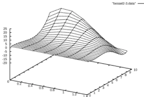
(3) Find the value f (b) by an adaptive Runge-Kutta method by the system of differential equations and the initial values at x = a. If we can find series solution at x = a and it converges at x = b rapidly, we may replace the last step by a computation of a series solution and its evaluation. As to methods to find series solutions, see the Chapter 2 of [18] and references of it, however there remains some fundamental unsolved problems. As a demonstration of our method, we close this paper with showing a graph of a solution of a Bessel differential equation in two variables [14], which is drawn by using our method (Figure 1).
"bessel2-3.data" 0 0.2 0.4 0.6 0.8 1 1.2 1.4 01 23 45 67 89 10 -20 -15 -10 -5 0 5 10 15 20 25
Figure 1. Bessel function in two variables: We consider the integral f (a; x, y) = R
Cexp(−14t2− xt − y/t)t−a−1dt, where C = ~01 + {e2π √
−1θ| θ ∈ [0, 2π]} + ~10. The
function f (a; x, y) satisfies the holonomic system ∂x∂y+ 1, ∂x2− 2x∂x+ 2y∂y+ 2a, 2y∂y2+
2(a + 1)∂y− ∂x+ 2x. The rank of the system is 3. Take a = 1/2. It admits a unique
solution of the form y−ag(x, y) such that g is holomorphic at the origin and g(0, 0) = 1.
This is the graph of g for (x, y) ∈ [0, 1.4] × [0, 9]. The function f (1/2; x, y) is a constant multiple of y−ag(x, y). The normal form computation in D is used to derive ODE’s to
apply for the adaptive Runge-Kutta method.
References
1. Almkvist, G., Zeilberger, D.: The method of differentiating under the integral sign. Journal of Symbolic Computation 10 (1990), 571–591. 2. Bernstein, J.: The analytic continuation of generalized functions with
re-spect to a parameter. Functional Analalysis and its Application 6 (1972), 273–285.
3. Castro, F.: Calculs effectifs pour les id´eaux d’op´erateurs diff´erentiels. Travaux en Cours, 24 (1987), 1–19.
4. Cox, D., Little, J., O’Shea, D.: Ideals, Varieties, and Algorithms, Springer, 1992.
5. Galligo, A.: Some algorithmic questions on ideals of differential operators. Lecture Notes in Computer Science 204 (1985), 413–421.
6. Kashiwara, M.: B-functions and holonomic systems, Inventiones Mathe-maticae 38 (1976), 33–53.
7. Kashiwara, M.: On the holonomic systems of linear differential equations, II. Inventiones Mathematicae 49 (1978), 121–135.
8. Noro, M.: An efficient modular algorithm for computing the global b-function, Mathematical Software, ICMS 2002 (2002), 147–157.
9. Oaku, T.: Computation of the characteristic variety and the singular locus of a system of differential equations with polynomial coefficients. Japan Journal of Industrial and Applied Mathematics 11 (1994), 485–497. 10. Oaku, T.: Algorithms for the b-function and D-modules associated with
a polynomial. Journal of Pure and Applied Algebra 117 (1997), 495–518. 11. Oaku, T.: Algorithms for b-functions, restrictions, and algebraic local
cohomology groups of D-modules. Advances in Applied Mathematics 19 (1997), 61–105.
12. Oaku, T., Takayama, N.: Algorithms for D-modules – restriction, tensor product, localization, and algebraic local cohomology groups. Journal of Pure and Applied Algebra 156 (2001), 267–308.
13. Oaku, T., Takayama, N., Walther, U.: A localization algorithm for D-modules, Journal of Symbolic Computation 29 (2000), 721–728.
14. Okamoto, K., Kimura, H.: On particular solutions of the Garnier systems and the hypergeometric functions of several variables. Quarterly Journal of Mathematics, 37 (1986), 61–80.
15. Oppenheim, A.V., Schafer, R.W.: Discrete-Time Signal Processing, Pren-tice Hall, 1989.
16. Petkovsek, M., Wilf, H.S., Zeilberger, D.: A = B. A K Peters, Ltd., 1996. 17. Press, W., Teukolsky, S., Vetterling, W., Flannery, B.: Numerical Recipes
in C++, Cambridge University Press, 1988.
18. Saito, M., Sturmfels, B., Takayama, N.: Gr¨obner Deformations of Hyper-geometric Differential Equations. Springer, 2000.
19. Takayama, N.: An algorithm of constructing the integral of a module, Proceedings of International Symposium on Symbolic and Algebraic Com-putation, (1990) 206–211.
20. Takayama, N.: Kan: A system for computation in algebraic analysis. Source code available at http://www.openxm.org Version 1 (1991), Version 2 (1994), The latest version is 3.021108 (2002).
21. Tamura, Y.: A design and implementation of a digital formula book for generalized hypergeometric functions, Thesis, (2003), Kobe University. 22. Wilf, H.S., Zeilberger, D.: An algorithmic proof theory for hypergeometric
(ordinary and ”q”) multisum/integral identities, Inventiones Mathemati-cae 108 (1992), 575–633.
23. Zeilberger, D.: A holonomic systems approach to special function identi-ties. Journal of Computational and Applied Mathematics 32 (1990), 321– 368.