Vol. 60, No. 2, April 2017, pp. 192–200
THE MATHEMATICAL MODEL OF PROJECT RISK RESPONSES IN PROJECT RISK MANAGEMENT
Hirokatsu Fukuda Hiroaki Kuwano
Kanazawa Gakuin University
(Received March 1, 2016; Revised January 4, 2017)
Abstract Project risk is an uncertain event that causes positive or negative effects on the project objectives in relation to the cost, time, quality and so on to complete the project. Project risk management is the set of processes of identifying, analyzing and responding to project risks. For example, the project risk management includes the process of eliminating the project risks from the project to complete any activities in the project by the specified day. In terms of not only the risk but also the time, many researches have been done. Especially, as for the time, there are many researches on CPM and PERT, which use mathematical techniques. However, few researchers discuss the effectiveness of project risk responses to deal with project risks for making a success of the project. In this paper, we propose a new mathematical model of the project risk responses. And, with our proposing model, we show how to calculate the effectiveness of project risk responses quantitatively. Moreover, we can decide quantitatively which project risk response should be executed by the consequences of the above calculation.
Keywords: Risk management, project management, project risk, project schedule
1. Introduction
As follows, project risk is defined by PMBOK Guide (a Guide to the Project Management Body of Knowledge) [9] presenting a set of standard terminology and guidelines for project management published by PMI (Project management Institute) that is the world’s leading association for the project management profession founded in 1969.
Project risk is an uncertain event or condition that, if it occurs, has a positive or negative effect on one or more project objectives such as scope, schedule, cost, and quality. A risk may have one or more causes and, if it occurs, it may have one or more impacts. A cause may be a given or potential requirement, assumption, constraint, or condition that creates the possibility of negative or positive outcomes.
By such project risks, some projects end in failure. On the other hand, we consider that some project risks can be controlled and following four strategies of project risk responses (the methods or measures to avoid and/or eliminate the risks’ damages) to deal with project risks are presented by PMBOK Guide [9].
Three strategies, which typically deal with threats or risks that may have negative impacts on project objectives if they occur, are: avoid, transfer, and mitigate. The fourth strategy, accept, can be used for negative risks or threats as well as positive risks or opportunities. Each of these risk response strategies have varied and unique influence on the risk condition. These strategies should be chosen to match the risk’s probability and impact on the project’s overall objectives.
We try to execute appropriate project risk responses in advance to lead the project to success. Project risk management is the set of the management processes that plan and execute the
project risk responses to control the project risks to complete the project successfully. However it is difficult to execute the appropriate project risk responses in the practical project under the existing conditions. That is, in many practical projects, the necessary project risk responses were not executed, so that some projects could not be completed within the periods of the projects and ended in failure. It is one of the reasons why projects end in failure that there are no means to evaluate the effectiveness of project risk responses quantitatively. Hence, the mathematical model is required to indicate the effectiveness of project risk responses.
There were many researchers used the traditional mathematical methods such as CPM or PERT, the project completion period has been studied that is the total number of days from the day that the first activity is started to the day that all activities in the project are completed [6–8].
The project completion period can be predicted with the estimations of the periods of all activities in the project. These researches have been providing the information about the project completion periods to lead the project to success for the decision-makers. More-over, the quantitative researches have been worked about the general risks, not just project risks [5, 10]. However with the information about the project completion period and those probability distributions, the decision-makers cannot choose the best project risk responses to lead the project to success. And, in recent years, Fukuda and his colleagues derive the new results about the effectiveness of the project risk responses in the framework of the project risk management [1–4]. One of their main results is the probability distribution of the increment of the project completion periods caused by the project risks. The proba-bility distribution is calculated with the estimations of the occurring probabilities and the consequences of the project risks, under the condition that all project risks which make effects on the project completion period can be identified. Still more the effects on the project completion periods by the project risk responses have not been studied yet by the quantitative researches about project risk management. Therefore there is a pressing need to give the decision-makers the effective information to choose the project risk responses appropriately.
2. Basic Concepts of Project Risk Management
In this section, we briefly review project, project risk, project risk management and project risk response.
First, project is the set of ordered activities and these activities have the periods to complete them. Project completion period is the total number of days from the day that the first activity is started to the day that all activities are completed. Each project has the target date and if the project can be completed before the target date, we consider the project ends in success and if it cannot, we consider it ends in failure.
Next, project risk is an event that causes the periods of some activities in the project longer than they were planned. Followings are some examples of project risks presented by PMBOK Guide [9].
For example, causes could include the requirement of an environmental permit to do work, or having limited personnel assigned to design the project. The risk is that the permitting agency may take longer than planned to issue a permit; or, in the case of an opportunity, additional development personnel may become available who can participate in design, and they can be assigned to the project. If either of these uncertain events occurs, there may be an impact on the project, scope, cost, schedule,
quality, or performance.
If a project risk occurs and the periods of some activities are increased, there are cases that the project completion period is increased and the project ends in failure. Therefore the
project risk is an uncertain event that causes the negative effects on the project completion
period and the consequence of the project if it occurs in this paper. The probability of a
project risk means the likelihood that the project risk will occur in the project and the consequence of a project risk or the number of delay days means the amount of increment
of the project completion period if the project risk occurs.
Project risk management means the whole process to manage project risks that cause
negative effects on the project objectives. For example, it means the process to eliminate identified project risks from the project to complete the project by the target date set in advance.
We assume that we can control the probabilities and the consequences of some project risks with the appropriate project risk responses in advance. Project risk response means such kind of actions to control the probabilities and the consequences of project risks. Project risk management includes the series of processes to identify the project risks that make effects on the consequence of the project, determine the appropriate project risk re-sponses and execute them. In this paper, we particularly focus on the project risk rere-sponses which control the number of delay days caused by some project risks.
3. The Mathematical Model of Project Risk Responses 3.1. The definition of project risk
In the practical project, a project risk might be intricately interrelated to the other project risks. So, it is very difficult to define practical project risks exactly. Then, we stand on the position that no project risk interact with the others. Project risk is defined as follows. Definition 3.1. Let (Ω,F, P) be the following probability space.
Ω ={r, rc}, F ={ϕ,{r}, {rc}, Ω}, P({r}) = p, P({rc}) = 1 − p, 0 < p < 1.
(1) We say r is project risk whose probability is p and cost is C, if the following two functions
S and C : Ω→ R exist. S(ω) = { 1, if ω = r, 0, if ω = rc , C(ω) = { d, if ω = r, 0, if ω = rc.
And the project risk r is denoted by r = ⟨S, p, C⟩.
(2) The probability space (Ω,F, P) is called the probability space associated with the project
risk r and the probability measure P is called the probability measure associated with the project risk r.
(3) The function S is called the status of the occurrence of the project risk r. The condition
of S = 1 represents that the project risk r occurs and the condition of S = 0 represents the project risk r doesn’t occur.
In the following discussions, we consider that the cost C of the project risk r is the number of delay days d > 0 that is the consequence of the project risk r, we regard C as
d and represent r = ⟨S, p, C⟩ as r = ⟨S, p, d⟩. Furthermore, we represent the project risk
whose probability is p and cost is C by the project risk r as an abbreviation.
We represent the K project risks by rk =⟨Sk, pk, dk⟩, k = 1, 2, . . . , K and the probability space associated with each project risk by (Ωk,Fk, Pk). And the set of indexes is denoted by U ={1, 2, . . . , K}.
A risk scenario that represents the occurrences of each project risk is defined in the following definition.
Definition 3.2. Let rk =⟨Sk, pk, dk⟩, k ∈ U be k project risks and (Ω, F, P) be the direct
product probability space of the probability spaces (Ωk,Fk, Pk) associated with each project
risk rk .
(1) The probability space (Ω,F, P) is called a probability space associated with a set of the
project risks RU ={rk, k ∈ U}.
(2) We say the following random variable S on (Ω,F, P) is a risk scenario of the set of
project risks RU for any ω = (ω1, . . . , ωK) ∈ Ω. S(ω) =(S1(ω1), . . . , SK(ωK)
)
∈ {0, 1}K
.
Remark 3.1. P(S = ℓ) is given by the following expression for any ℓ = (ℓ1, . . . , ℓK) ∈
{0, 1}K.
P(S = ℓ) = ∏ k∈U
Pk(Sk = ℓk).
The definition of a structure of project risks is given as follows.
Definition 3.3. Let (Ω,F, P) be the probability space associated with the set of project risks
RU ={rk=⟨Sk, pk, dk⟩, k ∈ U} and let S be its risk scenario.
(1) The vector d = (d1, . . . , dK) is called a risk impact vector of the set of project risks RU
where dk > 0 is the consequence of each project risk rk ∈ RU.
(2) We say (S, (Ω,F, P), d) is a structure of the set of project risks RU. 3.2. The definition of project
Project is defined in the following definition.
Definition 3.4. LetRU ={rk =⟨Sk, pk, dk⟩, k ∈ U} be the set of project risks, (
S, (Ω,F, P), d)
be its structure of project risks and let G = (V, E) be the directed graph with the source s∈ V and the sink t∈ V where each (i, j) ∈ E has the capacity uij > 0.
(1) We say P = (
(V, E),(S, (Ω,F, P), d), L
)
is a project with the delay limit L≥ 0.
(2) Each edge of G = (V, E) is called an activity and the capacity of each activity is called
an activity duration.
The number of delay days is defined in the following definition. Definition 3.5. Let P =
(
(V, E),(S, (Ω,F, P), d), L
)
be a project with the delay limit L ≥ 0. The random variable XU = S· d on (Ω, F, P) is called the number of delay days
with the set of project risks RU where · represents the canonical inner product. We express the project P =
(
(V, E),(S, (Ω,F, P), d), L
)
succeeds in the condition of
XU ≤ L and it fails in the condition of XU > L.
The above definitions give the general mathematical model for a project. However, we focus our discussion on a project that has only one activity in this paper.
3.3. The effectiveness of project risk responses
As shown in the previous sections, it is considered that we can avoid some project risks or decrease those magnitude of the negative effects with the appropriate project risk responses in the practical projects. In this section, we define a division of a structure of project risks to classify the project risks that are controlled by project risk responses and the project risks that are not controlled.
Let T ⊆ U be the set of indexes of the project risks that are controlled by project risk responses and set T ={1, . . . , m} (m < K) for the sake of simplicity. (ΩT,FT, PT) represents the probability space associated with the set of project risks RT ={rk =⟨Sk, pk, dk⟩, k ∈
T}, ST = (S1, . . . , Sm) represents the risk scenario and dT = (d1, . . . , dm) represents the risk impact vector. In the same way, (ΩU\T,FU\T, PU\T) represents the probability space associated with the set of project risks RU\T = {rk = ⟨Sk, pk, dk⟩, k ∈ U \ T }, SU\T = (Sm+1, . . . , SK) represents the risk scenario and dU\T = (dm+1, . . . , dK) represents the risk impact vector.
Furthermore, let XT = ST · dT be the number of delay days by the set of project risks
RT, XU\T = SU\T·dU\T be the number of delay days by the set of project risks RU\T. Then
XU\T represents the number of delay days of the project after the project risk responses have been executed and the set of project risks RT has been eliminated from the project.
It is supposed that XU = XT+XU\T is valid where XU, XT and XU\T are the numbers of delay days for each set of project risksRU, RT and RU\T. However, it is not valid because those random variables are defined on the different probability spaces.
Then let the random variables eXT and eXU\T be eXT = S· edT and eXU\T = S· edU\T with the K dimensions vectors edT = (d1, . . . , dm, 0, . . . , 0) and edU\T = (0, . . . , 0, dm+1, . . . , dK). And we similarly regard XT and XU\T as eXT and eXU\T if necessary. eXT and eXU\T are the independent random variables here.
The effectiveness of the project risk responses to avoid the set of project risks RT is represented as
P(XU\T ≤ L) − P(XU ≤ L) for the project P =
(
(V, E),(S, (Ω,F, P), d), L
)
of which the delay limit is L ≥ 0. From P(XU ≤ L) has been known, the quantitative effectiveness of the project risk responses can be evaluated with P(XU\T ≤ L).
Theorem 3.1. If P(XU ≤ x) and P(XT = x) are known for any x, P(XU\T ≤ L) can be
calculated by the following equations.
P(XU\T ≤ 0) = P(XU ≤ 0) P(XT = 0) , P(XU\T ≤ 1) = P(XU ≤ 1) − P(XT = 1)P(XU\T ≤ 0) P(XT = 0) , .. . P(XU\T ≤ L) = P(XU ≤ L) − L ∑ i=1 P(XT = i)P(XU\T ≤ L − i) P(XT = 0) .
P(XU = x), P(XT = x) and P(XU\T = x) represent the probability distribution of the
number of delay days with no project risk response, the probability distribution of the number of delay days caused by the set of project risks RT and the probability distribution of the
number of delay days with the project risk responses that eliminate the set of project risks RT from the project respectively.
Proof. By their definitions,
and, for any positive integer x, P(XU ≤ x) = x ∑ i=0 P( eXT = i)P( eXU\T ≤ x − i)
because eXT and eXU\T are independent random variables on the probability space (Ω,F, P). And P( eXT = 0) > 0 because 0 < pk < 1 for any k = 1, 2,· · · , K. Therefore, for x = 0
P(XU ≤ 0) = P( eXT = 0)P( eXU\T ≤ 0) , P( eXU\T ≤ 0) = P(XU ≤ 0) P( eXT = 0) . For x = 1, P(XU ≤ 1) = P( eXT = 0)P( eXU\T ≤ 1) + P( eXT = 1)P( eXU\T ≤ 0) , P( eXU\T ≤ 1) = P(XU ≤ 1) − P( eXT = 1)P( eXU\T ≤ 0) P( eXT = 0) . For x = L, P(XU ≤ L) = L ∑ i=0 P( eXT = i)P( eXU\T ≤ L − i) , P( eXU\T ≤ L) = P(XU ≤ L) − ∑L i=1P( eXT = i)P( eXU\T ≤ L − i) P( eXT = 0) .
We can regard XT and XU\T as eXT and eXU\T.
From Theorem 3.1, we can calculate the probability distribution of the increment of the project completion period caused by the project risks after the executions of the project risk responses. In practical project management, we calculate the probability distribution of the project completion period without any project risk responses by the Monte Carlo simulation with the estimations of the period of the activities in the project [9].
4. Numerical Example
In this section we illustrate that the appropriate project risk responses can be selected by the forecast of the probability distribution of the number of delay days with the project risk responses by using Theorem 3.1.
The probabilities and the number of delay days of the project risks in the project are shown in the table 1 and the delay limit of the project L = 20. The project risk responses can eliminate the project risk r1 or r2 from the project and we can choose r1, r2 or both of them to be eliminated from the project by the project risk responses. And we want to minimize the number of project risks to be eliminated under the condition that the success probability of the project is greater than or equal to 80%, that is P(XU\T ≤ L) ≥ 0.8.
The probability distribution of the number of delay days with no project risk responses is shown below. Additional project risk responses should be done, because P(XU ≤ L) = 0.69 < 0.8.
Project risks r1 r2 r3 r4 r5 r6 r7 r8 r9 r10 Probability 0.1 0.4 0.3 0.2 0.1 0.2 0.1 0.3 0.2 0.1 Number of delay days 15 10 0.3 0.2 0.1 0.2 0.1 0.3 0.2 0.1
Table 1: Probabilities and impacts of project risks
P(XU ≤ x) @ @ @ @ I
Number of delay days Probability
Target date
Figure 1: The probability distribution of the number of delay days with no project risk responses
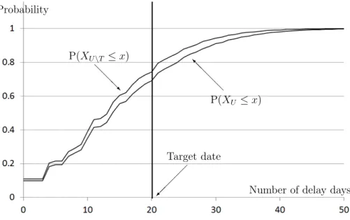
We calculate the number of delay days under the condition that the project risk r1 is eliminated from the project by the project risk responses using Theorem 3.1. Additional project risk responses should be done, because P(XU\T ≤ L) = 0.74 < 0.8.
P(XU ≤ x) @ @ @ @ I P(XU\T ≤ x) @ @ @ R
Number of delay days Probability
Target date
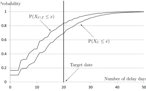
We calculate the number of delay days under the condition that the project risk r2 is eliminated from the project by the project risk responses using Theorem 3.1. Any additional project risk response is not necessary to be done, because P(XU\T ≤ L) = 0.84 ≥ 0.8.
P(XU ≤ x) @ @ @ @ I P(XU\T ≤ x) @ @ @ R
Number of delay days Probability
Target date
Figure 3: The number of delay days under the condition that r2 is eliminated We calculate the number of delay days under the condition that the project risks r1 and r2 are eliminated from the project by the project risk responses using Theorem 3.1. Any additional project risk response is not necessary to be done, because P(XU\T ≤ L) = 0.89 ≥ 0.8. P(XU ≤ x) @ @ @ @ I P(XU\T ≤ x) @ @ @ R
Number of delay days Probability
Target date
Figure 4: The number of delay days under the condition that r1 and r2 are eliminated Therefore, under the condition that the number of project risks to be eliminated should be minimized, it is appropriate that the project risk r2 is eliminated from the project by
the project risk responses. 5. Conclusions
In this paper, we derived the probability distribution of the number of delay days caused by the project risks after the executions of the project risk responses. It was calculated with the probability distribution of the number of delay days without any project risk responses and the probabilities/consequences of the project risks that would be eliminated from the project by the project risk responses. Besides, we showed the effectiveness of project risk responses was given quantitatively, using the probability distribution of the number of delay days after the executions of the project risk responses. This quantitative information about project risk responses make the decision-makers choose the appropriate project risk responses to lead the project to success.
Acknowledgements
The authors thank the anonymous referees and editors for constructive comments which improved this paper.
References
[1] H. Fukuda and H. Kuwano: On a generic framework of project risk. RIMS Koukyuroku, 1939 (2015), 162–171 (in Japanese).
[2] H. Fukuda and H. Kuwano: On a prioritization of project risks with the project risk model. The 2015 Spring National Conference of Operations Research Society of Japan
Abstracts (2015), 116–117 (in Japanese).
[3] H. Fukuda, H. Kuwano, and T. Shima: A study of delay time regarding project risk management. RIMS Koukyuroku, 1912 (2014), 112–120 (in Japanese).
[4] H. Fukuda, H. Kuwano, and T. Shima: A mathematical model of project risk and delay time. The 2014 Spring National Conference of Operations Research Society of Japan
Abstracts (2014), 184–185 (in Japanese).
[5] S. Kaplan and B. John Garrick: On the quantitative definition of risk. Risk Analysis, 1-1 (1981), 11–21.
[6] J.E. Kelley Jr: Critical-path planning and scheduling: mathematical basis. Operations
Research, 9-3 (1961), 296–320.
[7] K.R. MacCrimmon and C.A. Ryavec: An analytical study of the PERT assumptions.
Operations Research, 12-1 (1964), 16–37.
[8] J.O. Mayhugh: On the mathematical theory of schedules. Management Science, 11-2 (1964), 289–307.
[9] Project Management Institute: A Guide to the Project Management Body of Knowledge
(PMBOK Guide) (Fifth Edition) (Project Management Institute, Inc., 2013).
[10] M. Shaked and J.G. Shanthikumar: Stochastic Orders (Springer, 2006). Hirokatsu Fukuda
Kanazawa Gakuin University 10 Suemachi Kanazawashi Ishikawa 920-1392, Japan