APPLICATION OF PRINCIPAL COMPONENT ANALYSIS FOR PARSIMONIOUS SUMMARIZATION OF DEA INPUTS AND/OR OUTPUTS

(1)

Society of Japan

Vol. 40, No. 4, December 1997

APPLICATION OF PRINCIPAL COMPONENT ANALYSIS FOR

PARSIMONIOUS SUMMARIZATION OF DEA INPUTS

AND/OR OUTPUTS

Tohru Ueda Yoko Hoshiai

Seikei University NTT Laboratories

(Received August 4, 1995; Final June 12, 1997)

Abstract In Data Envelopment Analysis (DEA), when there are more inputs and outputs, there are more efficient Decision Making Units (DMus). For example, if the specific inputs or outputs advantageous for a particular DMU are used, the DMU will become efficient. Usually the variables used as inputs or outputs are correlated. Therefore, the inputs and outputs should be selected appropriately by experts who know their characteristics very well. People who are less familiar with those characteristics require tools to assist in the selection. We propose using principal component analysis as a means of weighting inputs and/or outputs and summarizing parsimoniously them rather than selecting them. A basic model and its modification are proposed.

In principal component analysis, many weights for the variables that define principal components (PCs) have negative values. This may cause a negative integrated input that is a denominator of the objective function in fractional programming. The denominator should be positive. In the basic model, a condition that the denominator must be positive is added. When the number of PCs is less than the number of original variables, a part of original information is neglected. In the modified model, a part of the neglected information is also used.

1.

Introduction

Data Envelopment Analysis (DEA) which was ingeniously developed by Charnes, Cooper and Rhodes

[3]

evaluates the relative efficiency of decision making units (DMU) that have many inputs and outputs. When there are more inputs and outputs, there are more efficient ones. For example, if the specific inputs or outputs advantageous for a particular DMU are used, the DMU will become efficient. Usually the variables used as inputs or outputs are correlated. Nunamaker

[6]

says that addition of a highly correlated variable may substan- tially alter the DEA efficiency evaluations. Therefore, the inputs and outputs should be selected appropriately by expert S who know their characteristics very well. People who are

less familiar with those characteristics require tools to assist in the selection. We propose using principal component analysis as a means of weighting inputs and/or outputs and summarizing parsimoniously them rather than selecting them. However, principal component analysis has two problems which have to be overcome. For these problems, a basic model and a modificaiton of it are proposed.

The first problem is as follows. In principal component analysis, many weights for the variables that define principal components (PCs) take negative values. This may cause a negative integrated input that is a denominator of the objective function in fractional programming.

If

both the numerator and the denominator have negative values, the fraction has a positive value, but it is difficult to compare the value with positive fraction values which are derived from positive numerators and positive denominators.

(2)

Appl~c;i;~on o f PCA for Parsimonious Summ. 467 In order to overcome this problem, fractions whose denominators and numerators are both negative must be transformed into appropriate forms. We conserve that the smaller inputs are, the better the efficiency is and also the more outputs are, the better the efficiency IS.

Even if denominators become positive by adding the same positive number, ordinal relations among denominators are conserved. When denominators are positive, ordinal relation among fractions can be always decided. From these, denominators must be positive. In the basic model, a constraint which satisfies this condition (Non-Negative Constraint: NNC) is added.

If all inputs are positive, NNC is redundant. However if there are negative inputs, NNC becomes effective. This means that in usual data the basic model is equivalent to models which do not have NNC and it can treat even negative inputs and outputs.

As the second problem, when the number of principal component is less than the number of original variables, a part of original informaiton is neglected as a variation factor. Mardia

51

says that principal component analysis looks for a few linear combinations which can be used to summarize the data, losing in the process as little information as possible. In the modified model, the information neglected in principal component analysis is recovered as much as possible.

2.

Parsimonious Summarization of Inputs and/or Outputs (Basic Model)

2.1

Basic model formulation

In this paper, DEA is discussed basically as fractional programming in the following way.

subject to

7;

_urOUTrj/

V

_{V ; I N P ; ;}

₅

₁_{( j}= 1 , 2 ,

,

n ) , r = l

i=

l

where

J

is the objective DMU,

I N P i j

is the i-th input of DMUj, and

OUTr.

is the r-th output of D M U j

( j

= 1 , 2 , .

.

,

n ) .

First we discuss the input variables. The same discussion applies for t h e outputs. If

INPij

=

I N P k j

(i

#

k

and

V j ) ,

v;

and

vk

cannot be determined uniquely in the same way as in regression analysis. Between highly correlated inputs,

v;

may b e unstable. Nunamaker

[6] says that methods for handling the variable selection are very important. If we use the principal components (PCs) as inputs in equation

(2.1),

they have no correlations. (See [4]

etc. for the principal component analysis.)

Let variables which have been usually used as input variables in DEA be

a;;,

and let their k-th PCs be

xk.

(3)

where G!' and S;(') are the mean and standard deviation of a;/'). In this standardization,

about half of the a;, have negative values, but the inputs used in equation (2.1) are desirable to be positive. It is known t h a t xkj in equations (2.2) and (2.3) do not change even if a constant c, is added to the original inputs a i / ~ ) / s i ( ~ ) . Letting c; equal G{'/si('), the following standardization is proposed instead of equation (2.4).

This is justified because of the coincidence of the origin point.

Let W k t = (wkl, wkb

,

wkm} be the weights used for the k-th principal components xk.

The inner products of different weight vectors equal zero. If all elements of w l are positive,

then half the elements of W ^ may be negative. This may result in negative denominators

in equation (2.1). T h e numerators in equation (2.1) are permitted to be negative, but the denominators are not. Thus, a constant CJ is added to the denominators in equation (2.1)

and the following constraints are

added

t o equation

(2. l),

where CJ is a constant depending on the objective

DMU

J.

Note that we cannot add the constants

d J

to the numerators in equation (2.1)~ because

DJ becomes close to one if all Ur and v, are very small and

CJ

= d ~ .

A

new formulation as

fractional programming for the target D M U J is rnax

subject t o _{u r ~ r j / ( x}_vkxkj

+

_CJ)

₅

_l_('j₌_l,_2,

_.

_.,

_n),

where is the k-th P C of

D M U j

for standardized inputs aij,

yrj is the r-th P C of D M U j for standardized outputs bhj, p

(<

m)

is the number of PCs for inputs, and

q

(<

S) is the number of PCs for outputs.

When the second condition in problem (2.7) is excluded, the following equation (2.8) is

a linear programming formulation of problem (2.7) and is called the output-oriented

BCC

model in Charnes et al.

[2].

P (2-8) min DJ =

X

i ^ x i . ~

+

CJ,

k= l q subject t o

_y'

_{u r ~ r J}= 1, r= l

(4)

Application o f PCA for Parsimonious Summ. 469 However, this equation cannot treat negative outputs, for example, for t h e case of ( q = 1) because of the first condition in this equation. Therefore, we propose the following model equivalent to problem (2.7) because of the second condition in the problem (2.7):

r = l P

subject to

X

_{u i x k ~}

+

_CJ

₌

_1,

k= l

Usually this model not only accords with t h e output-oriented

BCC

model (2.8) through linear transformation of uk and u r 7 and inverse of

D J ,

but also has solutions even in the case where the model (2.8) does not have any solutions.

We consider improvement of inefficient DMU. For t h e case in which outputs cannot be improved, the inputs of inefficient D M U J must be decreased. The left side of the second equation of equation (2.9) is expressed in terms of a i ~ as

where

Gi

= ukwki. k= l

Let

Il

be a set of improvable inputs of DMUJ,

I2

be a set of nonimprovable inputs of DMUJ, and a i ~ be the objective values

The must satisfy

(2.11) ViaiJ

+

CJ

i e h

2.2 Treatment

of

negative weights

of inputs a i ~ of D M U J for satisfying

{DJ

= l}.

T h e k-th

PC

xkt

= (xkl, xk2,

- ,

xkn) for inputs are given by equation (2.2). When there are many negative weights wki, the minimum weight

(<

0) has the same effect as the maximum weight

(>

0) in the principal component analysis. Therefore, evaluating the efficiency with absolute values of negative and positive weights is considered. Define

Pk,

Nk,

xkj^ and xt.fN) t o be

A

method of using both x k j ^ and x k j ^ may be considered, but it has the following shortcomings.

(a) The number of elements in

Nk

may be quite different from the number of elements in P k

(Nk

>>

P k or

Nk

<<

Pk).

(5)

(b) The effect of reducing the number of original inputs, m, to the number of PCs, p, is weakened.

(c) The discussion about PCs, for example, the contribution ratio, variance and so on, must be reconstructed.

(d) Suppose that all elements of w l are positive (NI is empty).

If

neither

Pi

nor

N2

is empty, the second input, x2j, is divided into two inputs, x2,^ and x2/"). This results in emphasizing x2 over

xi.

These points indicate that using xkj^ and xk/^ is not desirable. Considering that in the principal component analysis the first PC must be emphasized, the sign of the second and the following PCs for the inputs should be decided so that they have a positive correlation with the first PC for the outputs. The sign of the first P C for the inputs should be decided such that there are more positive xi,. The sign of PCs for the outputs should be decided in the same way.

2.3

Example

Here we present an application to a problem in the Nippon Telegraph and Telephone Corporation. A message area (MA) is an area in which users can talk by telephone for

3

minutes for 10 yen. The efficiency of 66 message areas was evaluated. The forty items shown in Table

1

were used as inputs and the following six items as outputs.

Revenue : Long distance,

blj

Local,

b2j

Numbers of subscribers : Business,

b3j

Residence, b4j

Public,

b5,

NTT

Business,

bgj

When DEA was applied directly to all inputs and outputs, the efficiencies of all DMus became one, because the number of inputs are too many for the number of DMus, considering that in Tone [l01 the following condition is requested:

where it is not always true that all efficiencies become one for such size of problems as this example. Then, the principal components

xi (i

= 1,2,

,

p) of the inputs and the principal components y k

(k

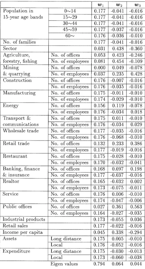
= 1 , 2 , - - - , q ) of the outputs were obtained. Weights w l , w2 and w3 in X I , x2 and x3 are shown in Table

1.

For outputs, the contribution ratio

C

Rl of the first PC is 0.998, and only the first

PC

was used as the

DEA

outputs, where

K

is a number of original variables

(K

= m for inputs) and

\,

is the j-th largest eigenvalue of a variance-covarience matrix of

K

variables. For inputs the contribution ratios of the first and second principal components are

0.794

and 0.064. Therefore, two PCs were used as DEA inputs.

In principal component analysis, (-wk) is not differentiated from wk. In DEA, (-W^) gives a different evaluation from wk. At first, the sign of weight vectors was decided such that there are more positive xki for each

k .

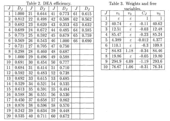
Table 2 shows the DEA efficiency

D J .

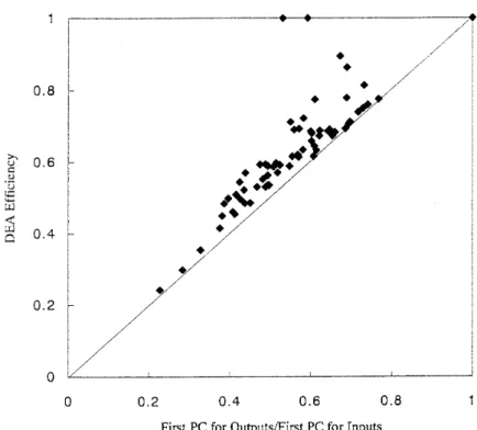
Figure

1

shows the first

PC

for outputs divided by the first PC for inputs versus DEA efficiency.

(6)

Application o f PCA for Parsimonious Summ.

Table 1. Weights.

1 A

l 1 l

Wholesale trade

1

No. of offices

1

0.177

1

-0.035

1

-0.016

No. of em~lovees

I

0.176

I

-0.068

I

-0.010

l l l

Population in 15-year age bands

No. of families Sector Agriculture, forestry, fishing Mining

&

quarrying Construction Manufacturing Energy Transport

&

communications l L " _l _l _l

Retail trade

1

No. of offices

1

0.132

1

0.233

1

0.386 0.177 0.177 0.177 0.177 0.176 0.177 0.031 0.053 0.081 0.000 0.037 0.176 0.176 0.175 0.174 0.156 0.176 0.175 0.176 0-14 15-29 30-44 45-59 60- No. of offices No. of employees No. of offices No. of employees No. of offices No. ofemployees No. of offices No. of employees No. of offices No. of employees No. of offices No. of employees - ~

Banking, finance

1

No. of offices

1

0.168

1

0.097

I

0.198 -0.041 -0.041 -0.041 -0.037 -0.036 -0.041 0.438 0.423 0.454 0.049 0.235 -0.007 -0.035 -0.011 -0.029 0.119 -0.034 0.011 -0.034 Restaurant

&

insurance

1

No. of employees

I

0.177

I

-0.037

I

-0.016 -0.016 -0.016 -0.016 -0.016 -0.010 -0.016 -0.360 -0.246 -0.109 -0.078 0.428 -0.016 -0.016 -0.010 -0.010 -0.078 0.018 -0.010 0.029 L No. ofemployees No. of offices No. ofemployees Eigen values 0.794 0.064 0.044 Realtor S er vi ce Public offices Industrial products Retail sales

Income per capita, Assets Expenditure 0.177 0.175 0.170 - No. of offices No. ofemployees No. of offices No. of employees No. of offices No. of employees Long distance Local Long distance Local -0.019 -0.028 -0.032 -0.016 -0.010 -0.041 0.165 0.173 0.176 0.174 0.027 0.164 0.173 0.177 0.045 0.175 0.176 0.175 0.173 -0.032 -0.075 0.006 -0.047 0.361 -0.027 -0.055 -0.022 0.338 0.005 -0.052 -0.030 -0.060 0.002 -0.011 -0.010 -0.006 0.563 -0.035 0.036 -0.016 -0.294 -0.010 -0.016 -0.013 -0.038

(7)

Table 2. DEA efficiency.

Table 3. Weights and free

The distance from the diagonal line represents the effect of the second P C for the inputs.

Table 3 shows weights vi, v2 and

U\

and free variables

CJ

in equation (2.9) for DMU1 to

DMU10.

All second PCs excluding MA (DMU)l for the inputs are positive, but the correlation

coefficients R(i, 1) between i-th P C for the inputs and the first P C for the outputs are

variables.

From the sign of R(2,

l ) ,

it may

be

considered t h a t

(-W^)

should be used instead of the

~k

used for Figure 1, but all second PCs excluding M A l , for the inputs become negative.

Considering that B(2,

l )

is very small, only the first P C should be used. Here, DMU1 is

J

1 a special DMU, having extremely larger (four to five times) inputs and outputs than the

second largest DMU and having the opposite sign of the second P C to other DMus as above

mentioned. This DMU1 is too large to compare with other DMus. Therefore, excluding

DMU1, analysis was also proceeded. In that case, the contribution ratio of the first P C for

output was 0.985. T h e contribution ratio of the first, second, and third PCs for inputs were

0.728, 0.057, and 0.053, so these three components were used as DEA inputs. Table 4 shows

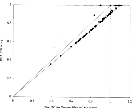
the weights and free variables and Figure 2 shows the first P C for outputs divided by the

first P C for inputs versus DEA efficiency when DMU1 is excluded. About half of

CJ

values

in Table 4 are positive and

CJ

does not have

a

bias toward negative, though all

CJ

except

for

(J

=

1)

in Table 3 are negative.

As a result we propose that t h e number of PCs should be decided according t o the

values of the contribution ratios

C R k

and the correlation coefficients R(i,

l )

and R(1,

jY

v1

E

after exclusion of D M u s with extraordinary inputs or outputs.

v2

E

c,

1 U 1

1

(8)

0 0.2 0.4 0.6 0.8 1

First PC for Outputs/First PC for Inputs

Figure 1. First PCs ratio versus DEA efficiency (including DMU1).

Table

4.

Weights and free variables (MA1 excluded).

3. Modified Model

When the number, p, of PCs is less than the number, m, of original variables and the

cumulative contribution ratio of p PCs is r ,

(1

- r) of total information is usually considered

as a variation factor, that is, a noise or a disturbance. In this section, the information (for

example, N I H l and N2H2 in Figure 3) is used positively and presented by one additional

dimension, t h a t is, total information is presented by (p

+

1)

dimensions.

3.1 Utilization of the mean and variance of a variation factor

When p PCs are x i , x2,

.

-

,

xp7 t h e ( p + l)-st variable

xp+l

with mean pp+1 and variance

Vp+l are added, where

(9)

0 0.2 0.4 0.6 0.8 1 1.2 First PC for Outputs/First PC for Inputs

Figure

2.

First PCs ratio versus

D E A

efficiency (excluding

D M U 1 ) .

Figure

3.

Perpendiculars from

N

to

H.

The k-th

PC,

{ x k t

=

( x k l , xk2,

-

,

x k n ) }

and its mean are given by

j=1

Considering that the sum of means of m standardized variables a: =

( a i l 7

,

sin)

[i

=

1 , 2 , - . - , m ]

is

i=l

P

and

(E

p k )

out of

it

is presented by p PCs, let pp+l be

(10)

Application of PCA for Parsimonious Summ. 4 75 Because pp+l and Vp+l do not depend on the

DMU, x p + ~

is expressed as a scalar variable xp+l. The same procedure as for the inputs is applied to the outputs, using the (q

+

l)-st variable, yq+l. T h e xp+1 and yq+l are supposed to be random variables. The following measure may come t o mind in place of the first equation in equation (2.7).

For the same reason that in Sec.2.1 no constant can be introduced in the numerators, the three parameters uq+1

,

and

CJ

cannot be used simultaneously. Therefore equation (3.5) cannot be used.

3.2 Consideration of the discrepancy between

P C space and the original space

Let the coordinates of a point,

N,

in vector space Vm be

Let the coordinates in Vm of the foot,

H,

of a perpendicular from

N

to the vector space Vp whose elements are p PCs be

(see Fig. 3). Because the number of PCs is limited to p, the vector of the values of m PCs at the point

H

is

x(H)

= (X^,,, X ~ H ,

,

_{X p H 1}_0,

.

,o)'.

Let

W

= ( w l , w 2 ,

. .

,

wm)',

X

= ( x i ,

x2,

-

,

xm)' and

A

= (01, 0 2 ,

- - - ,

a m ) t ,

where _wk= (wkl, w42,

-

.

,

wkm)' for

k

=

1 , 2 ,

.

,

m , especially, wh = 0 for

h

>

p,

xk = (xk1, x k 2 , .

.

,

x k a for

k

= l ,

2, - -

, m , and a k = (akl, a k 2 ,

- ,

aknlt for

k

= 1 , 2 ,

,

m.

Then,

Therefore, (3.10)

X

=

WA,

A

= W t X .

Considering t h a t fewer (aiA - is desirable, we hit on the idea that the denominator of the first equation in equaiton (2.7) may be changed to

This compensates the reduction in information of PCs. Here, from the viewpoint of pa- rameter parsimony, individual parameters, up+;, should not be taken for each (ai7 - a;,/^).

Applying this idea t o the outputs as well as the inputs, the following modified model is proposed instead of equation (2.7). In this model, (p

+

2) variables, [vl, v2,

- ,

vp+l, C'J], for inputs and (q

+

1)

variables, [ul, u2,

,

u ~ + ~ ] , for outputs must be decided.

(11)

[Proposed Model]

max

9 S P m

D ~ 2 =

{'E

U ~ Y ~ J

+

~ q + l

E(bi~

- b i j ( H ) ) } / { ~ i x i J

+

up+l

Y , ( ~ ~

- a i J ( ~ ) )

+

C.,},

subject to

where

bij

and

h i / '

are defined in the same way as aij and ai/^.

Figure

4

shows the relation between the first P C of outputs divided by the first P C of inputs and the efficiency, DJ2, where DMU1 was excluded and {p = l , q = l}. Figure 4 has a slightly larger variation above the lowest line than Figure

2.

First PC for Outputs/First PC for Inputs

Figure

4.

First PCs ratio versus DEA efficiency, DJ2 (excluding DMU1)

3.3

Improvement of inputs in the modified model

This section discusses the improvement of inputs in the modified model of Sec.3.2 for the case in which outputs cannot be improved on the lines of equation (2.11). Suppose that every input, U ~ J , of an inefficient DMUJ is decreased at a constant rate,

K

(<

l ) , to

(12)

that is,

hJ

is also decreased at rate

I{.

Moreover,

Therefore, if

then DJ2 = 1.

4. Conclusion

We proposed t h a t the sign of PCs for the inputs (outputs) should be decided according to the correlation coefficients between those PCs and the first P C for outputs (inputs), and that the number of PCs should be decided from the values of the contribution ratios, C R h and the correlation coefficients, R(i, 1) and R(1,

j ) .

We presented a basic model and a modification of it t h a t takes factors unexplained by PCs into account.

We overcame the disadvantage of principal component analysis and made possible its use as a parsimonious summarization tool for DEA inputs and/or outputs. Of course, we do not use principal component analysis when the inputs or outputs are not so many and the correlations among the inputs or outputs are weak.

The number, p, of principal components is usually decided by the commulative contribution ratio,

CC

RP, or t h e p-th eigenvalue, Ap. The more the value of p is, the more difficult it is to explain the meaning of each principal component. Therefore, we propose limiting p to the small values and recovering information with a modified model shown in Sec.3.2. From references [4],

[5],

[7]

and

181,

we recommend CCR,

2

0.7

or

A,

2

1

for correlation matrix. If the modified model is used for (p -

1)

PCs, we can derive a model that has the same number of variables and does not neglect completely information which is presented by residual (m - p

+

1) PCs. This model becomes a compromise between t h e basic model in

Sec.2 and models which use all variables. For the modified model there may be other ideas and we need further study.

If variables are classified into some groups whose members have a high correlation each other and t h e principal component analysis is applied to each group, intuitive interpretation of results becomes easy, but a number of inputs or outputs may not decrease very much.

In multivariate analysis, canonical correlation analysis is well-known as a means of an- alyzing two sets of variables. In this paper, they are a set of input variables and a set of output variables. Let the i-th canonical variables for inputs and outputs be f i and g,, respectively. Canonical correlation analysis has shortcomings as a method of summarizing parsimoniously variables and evaluating efficiency in DEA. For example, there is no correlation between f 2 and gl. We cannot explain any meanings of the linear combination of

fi

and f2. T h e fractional programming which has f2 in denominator and 91 in numerator

should not be approved. When as a measure of efficiency, we only use a ratio, g l /

f l

,

of the first canonical variables, canonical correlation analysis may have some meanings.

In equation (2.9) a non- Archimedean infinitesimal E was introduced. We can derive an c-free DEA in the same way as a 2-phase process in Tone

[g].

In the similar way we can also derive a n E-free DEA for equation (3.11).

We discussed DEA as a fractional programming problem and added constraints that denominators must be positive. Discussion in negative weights and modified models are also applicable to other formulations of DEA. Especially, for the purpose that we do not

(13)

mind signs of inputs, it may be appropriate to use additive DEA models (see Charnes et al.

[l]). References

[l]