修 士 論 文 の 和 文 要 旨
研究科・専攻 大学院情報理工学研究科 情報・ネットワーク工学専攻 博士前
期課程
氏 名 Boungnong Nilandone 学籍番号 1831133
論 文 題 目 Window size optimization of Hidden Markov Item Response Theory (隠れマルコフ項目反応モデルにおけるウィンドウサイズの最適化) 要 旨 近年,大規模公開オンライン講座を始めとする e ラーニングシステムが大きな注目を集 めている.しかし,多くの e ラーニングシステムは動的に学習者の知識状態を推定し,学 習者に適応した支援をすることができていない.そのため,学習者の知識状態を推定する モデルの開発が大きな課題となっている.学習者の知識状態を推定する手法の一つに隠 れマルコフ項目反応理論(HMIRT)が存在する.HMIRT は一般の項目反応理論(IRT)を 時系列に拡張したモデルであり,以下の二つのパラメータを持つ.1)知識状態が過去の学 習データにどれだけ依存するかを決定できるウィンドウサイズパラメータ.2)学習者の 知識状態の変動幅を決定する分散パラメータ.既存の HMIRT では,これらのパラメー タが全ての時点に共通する,あらかじめ決定された固定パラメータであった.しかしなが ら,知識状態が過去の学習データにどの程度依存するかは取り組む項目によって異なる ため,ウィンドウサイズパラメータを固定することで知識状態の推定精度が損なわれて いる恐れがある.さらに,分散パラメータを固定することで,学習者の知識状態の変動が 全ての時点で一定となることもモデルの表現力を制限している. 本研究では,これらの問題点を解決するために,ウィンドウサイズパラメータを各時点で 変動できるよう拡張した HMIRT モデルを提案する.具体的には,貪欲法を用いて各項 目ごとに最適なウィンドウサイズパラメータを推定する. 評価実験では,実データを用いて従来の HMIRT モデルと提案モデルについて,未知の 課題への反応予測精度を比較した.その結果,提案手法は既存手法と比較して高精度に未 知の課題を予測できることが明らかとなり,ウィンドウサイズパラメータを各時点で変 動させることが有効であることが示された.
2
令和二年度 修士論文
Window size optimization of Hidden Markov Item Response
Theory
電気通信大学 大学院情報理工学研究科
情報・ネットワーク工学専攻 情報数理工学プログラム
学籍番号 1831133
Boungnong Nilandone
主任指導教員 植野 真臣教授
指導教員 川野 秀一 准教授
提出年月日 2021 年 1 月 25 日
Table of Contents
1. Introduction ... 1
2. Item Response Theory (IRT) ... 4
3. Hidden Markov Item Response Theory (HMIRT) ... 6
4. Auto-Fluctuation Window Size HMIRT (AFHMIRT) ... 10
5. Parameter Estimation ... 12
6. Experiment ... 16
6.1. Response Prediction Accuracy ... 17
6.2. Window Size Parameter ... 21
6.3. Variance Parameter ... 23
7. Conclusion ... 25
Table of Figures
Fig 1 Traditional Item Response Theory model………...5
Fig 2 Representation of Hidden Markov Item Response Theory model ………...6
Fig 3 Response prediction accuracy for each Window Size of Foundation of Programming 1 (7 tasks, 148 learners, δ=0.7)………..………8
Fig 4 Response prediction accuracy for each Window Size at each task of Foundation of Programming 1 (7 tasks, 148 learners, δ=0.7)………...………8
Fig 5Example of an Auto-Fluctuation Window Size HMIRT model………11
Fig 6 Response prediction accuracy of Foundation of Programming 1……….……...19
Fig 7 Response prediction accuracy of Foundation of Programming 1……….……...20
Fig 8 Response prediction accuracy of Information Society and Information Ethics……….……….20
Fig 9 Window Size of Foundation of Programming 1 ……….21
Fig 10 Window Size of Foundation of Programming 2……….22
Fig 11 Window Size of Information Society and Information Ethics……….22
Fig 12 Variance of Foundation of Programming 1. ……….23
Fig 13 Variance of Foundation of Programming 2…….……….24
Fig 14 Variance of Information Society and Information Ethics……….24
Table 1: Average Response prediction accuracy………..………...18
1
1. Introduction
In recent years, learning assistance has been gaining more attention in the education field.
Because over-instruction or under-instruction can lead to ineffective knowledge development, determining the amount of support that a learner needs has been a major
challenge for educators. Vygotsky (1962) introduced the Zone of Proximal Development (ZPD) for problem solving, where a learner cannot solve difficult tasks alone but can do so with an expert’s help, thereby promoting learner development [1][2]. Using the ZPD
concept, Wood et al. (1976), Collins (1989), and Bruner (1996) have shown that when
learners face higher-level tasks, the teachers should provide moderate support depending on the learner’s ability through the process of “scaffolding” [3][4][5]. Scaffolding is a
process where the learners obtain support to solve tasks that are beyond their capability when solving by themselves.To provide optimal help for scaffolding learners, Ueno and
Matsuo [6] proposeda scaffolding system that predicts the learner’s performance. In other words, to effectively assist the learner, their knowledge and their performance must be
accurately estimated.
To estimate the learner’s knowledge, Ueno and Matsuo [6] and Ueno and Miyazawa
[7][8] proposed the use of Item Response Theory (IRT). IRT is one of the test theories that can be used to estimate the learner’s ability based on past learning data and can also
be used to predict the response of the learner by calculating the probability of getting a correct answer based on the learner’s estimated ability [9]. However, IRT assumes that each task is dependent on a static learner’s ability, meaning that the learner’s ability does
not change during the learning process, which might lead to inaccurate prediction of the learner’s response.
2
To handle the change in the learner's ability during the learning process, Tsutsumi et al.
(2019) [10][11] proposed the Hidden Markov Item Response Theory (HMIRT) model, which treats the learner's ability as a time-series. HMIRT assumes that at some point
during the learning process, the learner will gradually forget about past tasks. HMIRT uses the Sliding Window method to model the learner forgetting about the earlier tasks. HMIRT also assumes that the learner’s ability to perform each task does not change before
the point at which the learner forgets, meaning that these tasks will be dependent on one value for the learner’s ability, the same as in the traditional IRT. After a learner increases
his/her ability due to the learning effect, the learner's ability will be updated and used in
the next task. To handle this process, HMIRT introduces two new parameters: the window size parameter is a fixed number used to control how many of the previous tasks affect the estimation of the learner’s current ability, and the variance parameter is a fixed number
used to control the magnitude of change in the learner’s ability at each time point. This
model fixes the problem of static ability in the traditional IRT model, leading to more accurate estimation of learner’s ability and therefore performance.
It has been shown that HMIRT estimates the learner’s ability better than the traditional
IRT [10][11]. However, HMIRT’s constant window size might not guarantee an accurate estimation of learner’s ability. Another limitation of HMIRT is the fixed variance
parameter. Setting a fixed variance parameter limits the change in the learner’s ability at each time state. If the variance parameter is small, the learner’s ability will not change
much. If the variance parameter is large, the learner’s ability will change too much.
Because the content of each task varies, the degree of understanding gained by completing each task must also be different. Therefore, accurate prediction cannot be guaranteed
3
when using a fixed variance parameter. To solve these problems, we propose the
Auto-Fluctuation Window Size of Hidden Markov Item Response Theory Model. In this model, the window size and variance parameters are time series rather than fixed values so that
the parameters can change at each time point. With this proposed model, we expected a more flexible and more accurate estimation of learner’s ability.
4
2.
Item Response Theory
To effectively support the learner’s development, learner performance prediction is
needed. To predict a learner's performance, Item Response Theory (IRT)[9][12] has been used. IRT is one of the test theories based on mathematical models and has been used
widely in computer testing. It has the following advantages:
1. It is possible to assess ability while minimizing the effect of the heterogeneous
or aberrant items, which has a low estimation accuracy.
2. The learners’ responses to different items can be assessed on the same scale.
3. Missing data can be readily estimated.
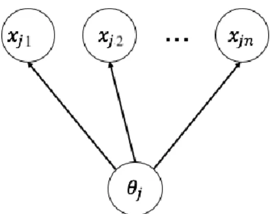
In the IRT model, one of the most used models is the two-parameter logistic model (2PL). In the dichotomous response, 𝑥𝑗𝑖 denotes the response of the learner 𝑗(1, . . , 𝑛) to 𝑖-th
item as:
With the learner’s ability variable 𝜃𝑗, 2PL can be expressed by:
𝑃(𝑥𝑗𝑖 = 1|𝜃𝑗, 𝑎𝑖, 𝑏𝑖) = 1
1 + 𝑒𝑥𝑝{−1.7𝑎𝑖(𝜃𝑗− 𝑏𝑖)}
where the item parameter 𝑎𝑖 and 𝑏𝑖 is called the discrimination parameter and difficulty parameter, respectively, 𝜃𝑗 is the latent ability variable of learner 𝑗. The item
parameter 𝑎𝑖, 𝑏𝑖 was estimated in advance from the training data. 1: correct response for 𝑖-th item
0: incorrect response for 𝑖-th item 𝑥𝑗𝑖 =
5
In this model, because all of the items depend on one prior distribution of ability variable,
the estimation of the ability variable is less affected by the prior distribution but is easily affected by the learning process. Therefore, the over-training occurs and the ability
variable might be overly estimated or underestimated.
In order to avoid the over-training, Tsutsumi et al. [10][11] proposed the Hidden Markov
model, which changes the learner’s ability to time-series where the current ability variable depends on the value of previous ability variable. With this model, the accuracy of the learner’s ability estimation has been improved.
6
3. Hidden Markov Item Response Theory
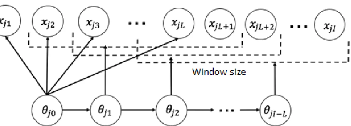
The Hidden Markov Item Response Theory (HMIRT) model is an extension of the IRT model that replaces the fixed value for the learner’s ability 𝜃𝑗 with the time-series 𝜃𝑗𝑡, where the change in ability at time 𝑡 depends on the value of the ability variable 𝜃𝑗𝑡−1
at time 𝑡 − 1 according to a Hidden Markov process. Here, the number of task items used in the ability estimation at time 𝑡 has been set, denoted by L. HMIRT assumes that
the value of the ability variable does not change for items 𝑖 = 1, … , L, which means that these initial items will depend on the same ability value (as in the IRT model). When the item 𝑖 > L, the ability variable 𝜃𝑗𝑡 will change based on 𝜃𝑗𝑡−1. The variance parameter 𝛿 must be estimated to control the transition (amount of variation) of the ability variable 𝜃𝑗𝑡 between each time state.
The transition model for the ability variable 𝜃𝑗𝑡(𝑡 = 1, … , 𝐼 − 𝐿) uses the sliding
window method [13][14].The sliding window is a method of determining the number of hidden variables that will affect the ability estimation when shifting by the set window
size. When the current item 𝑖 > L, the ability estimation is conducted by shifting the window along the items one at a time (Figure 2).
7
In this model, the number of items that depends on one ability variable in each learning
process is defined by the window size parameter L. The learning process at time 𝑡 is as follows: { 𝑡 = 0: 𝑖 = 1, … , 𝐿 𝑡 = 1: 𝑖 = 2, … , 𝐿 + 1 ⋮ 𝑡 = 𝐼 − 𝐿: ⋮ 𝑖 = 𝐼 − 𝐿, … , 𝐼
When L is small, only the learner's most recent history will influence their estimated ability 𝜃𝑗𝑡. If L is larger, additional task items will factor into the ability estimation.
This model was originally developed for the dynamic assessment system, which gives hints to the learners when they cannot solve the task. In this research, we generalize the model so that it can work without the hint. The probability 𝑃𝑖𝑗𝑡 of a correct answer for task item 𝑖 being provided by learner 𝑗 based on their ability 𝜃𝑗𝑡 at time 𝑡 is as
follows: 𝑃𝑖𝑗𝑡 = 1 1 + 𝑒𝑥𝑝 (−𝑎𝑖(𝜃𝑗𝑡− 𝑏𝑖)) where 𝜃𝑗𝑡 ~ 𝑁(𝜃𝑗𝑡−1, 𝛿) 𝜃𝑗0 ~ 𝑁(0,1)
𝛿 is the variance parameter, which controls how much the estimated ability can change
during each learning session. In this model, the window size parameter L and the variance
parameter 𝛿 perform important roles in the prediction of the learner’s performance. (3) (3) (3) (3) (3) (4) (4) (4) (4) (5) (5) (5) (5) (2) (2) (2) (2) (2) (2) (2) (2) (2)
8 0.66 0.68 0.7 0.72 0.74 0.76 2 3 4 5 6 7 Re spo nse pr ed ic tion A cc urac y Window Size
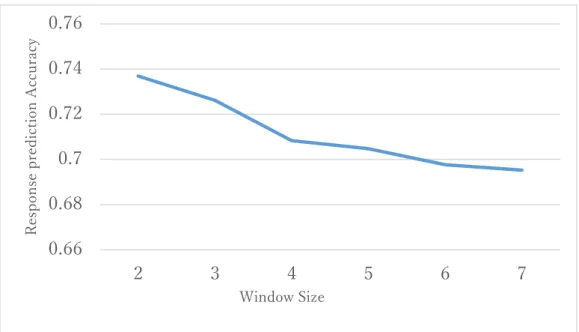
Fig. 3 Response prediction accuracy for each Window Size of Foundation of Programming 1 (7 tasks, 148 learners, 𝜹=0.7).
Fig. 4 Response prediction accuracy for each Window Size at each task Foundation of Programming 1 (7 tasks, 148
learners, 𝜹=0.7). 0.4 0.5 0.6 0.7 0.8 0.9 2 3 4 5 6 7 Re spo nse pr ed ic tion A cc urac y Window Size Task 2 Task 3 Task 4 Task 5 Task 6 Task 7
9
Figure 3 shows the response prediction accuracy for each Window Size of the dataset
Foundation of Programming 1(Ueno,2004) [15]. From Fig.3, we can see that the response prediction accuracy of HMIRT where the Window Size is two gets the highest value. On
the other hand, the traditional IRT (Window Size is seven) gets the lowest accuracy.
However, from Figure 4, when we look at each task separately, we can see that when the
Window Size is two do not guarantee the highest response prediction accuracy for all the tasks. From the result shows in Fig.4, we can say that HMIRT’s fixed window size may not guarantee an accurate estimation of learner’s ability, since the previous tasks that
contribute to the ability estimation at each time state can vary for the current task.
Moreover, setting a fixed variance parameter limits the range of transition of the learner’s ability at each time state. To solve this problem, the Auto-Fluctuation Window Size of
10
4. Auto-Fluctuation Window Size HMIRT
In the previous researches [10][11], it has been shown that the response prediction of
HMIRT is more accurate than that of traditional IRT. Fig.3 shows that the highest average response prediction accuracy is when the window size equals two. However, by observing
the response prediction accuracy rate for each task in Fig.4, we found that the window size equals two does not guarantee to obtain the highest response prediction accuracies at
each task. With this fact, we can assume that in some cases, changing the window size can lead to a more accurate estimation of learner’s ability. Moreover, the fixed variance parameter in HMIRT limits the range of transition of the learner’s ability at each time
state. Because the content of each task varies, the degree of understanding gained during
that task must also be different. Therefore, making the variance parameter changeable at each time point can lead to a more accurate learner’s ability estimation. To handle the
changes in the window size and variance parameters at each time state, we propose the Auto-Fluctuation Window Size HMIRT (AFHMIRT) model.
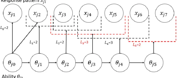
The AFHMIRT model replaces the fixed values for the window size parameter L and variance parameter 𝛿 with the time-series window size 𝐿𝑡 and variance parameter 𝛿𝑡
where 𝑡 is the time state of the learning process. The model then estimates the window size 𝐿𝑡 and the variance 𝛿𝑡 that maximize the response prediction accuracy for each
task. In the response prediction process of the HMIRT model, the system first estimates the item parameters, then estimates the learner’s ability for all of the time states 𝜽𝑗, then
finally calculates the response prediction accuracy. Because we want to find the optimal window size and variance for each item, we need to calculate the response prediction
11
parameters and the learner’s ability for only the current time state, then calculate the
response prediction accuracy for one item at a time while adjusting the window size and the variance to find the optimal window size for that item. When adjusting the window
size and the variance, the model needs to re-estimate the item parameters and the learner’s ability because these changes affect the calculation of the likelihood that will be used in
parameter estimation. After re-estimating the parameters, the response prediction accuracy is re-calculated. The learning process at each time state can be written as
follows: { 𝑡 = 0: 𝑖 = 1, … , 𝐿0 𝑡 = 1: 𝑖 = 2, … , 𝐿1+ 1 ⋮ 𝑡 = 𝐼 − 𝐿𝑡: ⋮ 𝑖 = 𝐼 − 𝐿𝑡, … , 𝐼
Figure 5 is an example of how the model will look when obtaining the optimal window size parameter for each item. For a 7-item model, 𝐿𝑡={2,2,2,3,3,2}.
(6) Fig. 3 Exa mpl e of an Aut o-Flu ctu atio n Wi ndo w Siz e Fig. 5 Example of an Auto-Fluctuation Window Size HMIRT model
12
5. Parameter Estimation
One of the popular methods for estimating item parameters for the IRT model is to use
the expectation-maximization (EM) and Newton-Raphson algorithms to estimate the marginal maximum likelihood (MML). The other method is maximum a posteriori
(MAP) estimation. For both MML and MAP estimation, when the method is applied in a simple model such as a two-parameter logistic model or a grade response model, or when
the dataset is large, the parameter estimation will be stable and accurate. On the other hand, when dealing with a complex model or when the dataset is small, the accuracy of
the parameter estimation will be decreased. In recent years, the use of the Markov Chain Monte Carlo (MCMC) method to estimate the expected a posteriori (EAP) for parameter
estimation has become more common. The MCMC method generates a random sample from the parameter’s posterior distribution and uses the generated sample to estimate the parameter’s expected value. In this research, we decided to use the MCMC method for
parameter estimation because this method is better suited to the limited dataset and more
complex model. In MCMC, there are many methods of generating a random sample; in this research, we use Metropolis-Hastings within a Gibbs algorithm. With the parameter 𝜃 = {𝜃10, … , 𝜃𝑗𝐼−𝐿}, 𝑎 = {𝑎1, … , 𝑎𝐼}, 𝑏 = {𝑏1, … , 𝑏𝐼} and the prior distribution 𝑔(𝜃𝑗𝑡|𝛿𝑡), 𝑔(𝑎𝑖), 𝑔(𝑏𝑖), given the response pattern 𝑋, the posterior distribution of the
parameters can be expressed as follows: 𝑝(𝜃, 𝑎, 𝑏|𝑋) ∝ 𝐿(𝑋|𝜃, 𝑎, 𝑏)𝑔(𝑎)𝑔(𝑏)𝑔(𝜃) = [∏ ∏ (𝑃𝑖𝑗𝑡)𝑥𝑖𝑗(1 − 𝑃𝑖𝑗𝑡)1−𝑥𝑖𝑗 𝐿+𝑡+1 𝑖=𝑡+1 𝐼−𝐿 𝑡=0 ] [∏ 𝑔(𝑎𝑖)𝑔(𝑏𝑖) 𝐼 𝑖=1 ] [∏ ∏ 𝑔(𝜃𝑗𝑡) 𝐽 𝑗=1 𝐼−𝐿 𝑡=0 ] (7) (7)
13 where Log 𝑎𝑖 ∼ 𝑁(0.0, 0.2) 𝑏𝑖~𝑁(0.0, 1.0) 𝜃𝑗0 ∼ 𝑁(0.0, 1.0) 𝜃𝑗𝑡 ∼ 𝑁(𝜃𝑗𝑡−1, 𝛿𝑡)
Let 𝜃′𝑗 be the current parameter value for 𝜃𝑗𝑡 = (𝜃𝑗0, … , 𝜃𝑗𝐼−𝐿) and 𝜃𝑗 be a new
proposal for the parameter obtained by the following: 𝜃𝑗 ∼ 𝑁(𝜃′𝑗𝑡−1, 0.01)
The acceptance rate for the parameter sampling is then as shown below:
𝛼(𝜃𝑗|𝜃𝑗′) = min (𝐿(𝑋𝑗|𝜃𝑗, 𝑎 ′, 𝑏′) ∏ 𝑔(𝜃 𝑗𝑡) 𝐼−𝐿 𝑡=0 𝐿(𝑋𝑗|𝜃′𝑗, 𝑎′, 𝑏′) ∏ 𝑔(𝜃′ 𝑗𝑡) 𝐼−𝐿 𝑡=0 , 1)
The same formula is applied for parameter sampling of 𝑎𝑖 and 𝑏𝑖. .
In this research, we set the MCMC maximum chain length to 40,000 iterations. To
eliminate the effect of the initial value, we set a burn-in period of 20,000 iterations. After the burn-in period, a sample is collected for an interval of 1000 iterations, and the average
is taken to be the EAP estimation value. Pseudo-code for the parameter estimation is shown in Algorithm 1. (8) (8) (8) (8) (8) (8) (8) (8) (8) (9) (9) (9) (9) (9) (9) (9) (9) (10) (10) (10) (10) (10) (10) (10)
14 Algorithm 1 Parameter Estimation with MCMC Given maximum chain length S,burn-in B,interval E Initialize MCMC sample 𝐴 ← ∅
Initialize 𝜃0, 𝑎0, 𝑏0 for 𝑠 = 1 to 𝑆 do for 𝑗 ∈ {1, … , 𝐽} do
Sample 𝜃𝑗𝑠 ∼ 𝑁(𝜃𝑗𝑠−1, 0.01)
Accept 𝜃𝑗𝑠 with the probability 𝛼(𝜃𝑗|𝜃𝑗′) end for
for 𝑖 ∈ {𝑡 + 1, … , 𝑡 + 1 + 𝐿𝑡} do Sample 𝑎𝑖𝑠 ∼ 𝑁(𝑎𝑖𝑠−1, 0.01)
Accept 𝑎𝑖𝑠 with the probability 𝛼(𝑎𝑖|𝑎𝑖′) Sample 𝑏𝑖𝑠 ∼ 𝑁(𝑏𝑖𝑠−1, 0.01)
Accept 𝑏𝑖𝑠 with the probability 𝛼(𝑏𝑖|𝑏𝑖′) end for if 𝑠 ≥ 𝐵 𝑎𝑛𝑑 𝑠%𝐸 = 0 then 𝐴 ← (𝜃𝑠, 𝑎𝑠, 𝑏𝑠) end if end for return average of A
From Fig.4, we can see that the response prediction accuracy at each task is not sorted by the Window Size. To estimate the window size parameter 𝐿𝑡 that maximizes the
response prediction accuracy, we propose the use of the linear search algorithm. The linear search algorithm is a method for finding an element within a list. It sequentially
checks each element of the list until a match is found or the whole list has been searched. The optimal variance parameter 𝛿𝑡 is also obtained by linear search algorithm for 𝛿 = {0.1, … ,1.0}, then taking the variance with the maximum response prediction accuracy.
The process of estimating the window size parameter 𝐿𝑡 and variance parameter 𝛿𝑡
15
Algorithm 2 Window Size and Variance Parameter Estimation with Linear Search Given Task number I
Initialize Window Size 𝐿𝑡,variance 𝛿𝑡 for 𝑖 = 0 to 𝐼 do
for 𝑙 = 2 to 𝐼 do
for 𝛿 ∈ {0.1, … ,1.0} do
Calculate response prediction accuracy with 𝑙 and 𝛿 𝐿𝑡← 𝑙 with maximum response prediction accuracy 𝛿𝑡 ← 𝛿 with maximum response prediction accuracy end for
end for end for return 𝐿𝑡, 𝛿𝑡
16
6. Experiment
To evaluate the estimates of learner’s ability produced by the proposed model, the
learner’s ability parameter was estimated, then used to predict the learner's response.
After obtaining the predicted response, the response prediction accuracy was calculated
using the real test data, and the results were compared with those of the HMIRT model and traditional IRT model. The data used in this study consisted of a number of learning
tasks within three courses:
(1) Foundation of programming 1 (7 tasks, 148 learners)
(2) Foundation of programming 2 (18 tasks, 75 learners)
(3) Information Society and Information Ethics (13 tasks, 23 learners)
These data are taken from the SAMURAI e-learning system for university students (Ueno,2004) [15]. We performed 10-fold cross-validation in the experiment to reduce
over-fitting and generalize the response prediction accuracy.
In addition, to evaluate the proposed model, the F-Measure and the Area under the curve
(AUC) were calculated.
The setting for the HMIRT model is as below[10][11].
(1) Foundation of programming 1: window size equals 2, δ equals 0.7
(2) Foundation of programming 2: window size equals 3, δ equals 0.4
(3) Information Society and Information Ethics: window size equals 2, δ
equals 1.0
For the traditional IRT model, the window size is equal to the task number, δ is equal
17
6.1. Response Prediction Accuracy
After obtaining the learner’s ability, the response for each item can be predicted by
calculating the probability of the learning getting the correct answer using equation (1) and then setting the response as follows:
After obtaining the predicted response for each item, it is checked against the real response data, and overall response prediction accuracy is calculated by taking the
average accuracy of all of the items. Here, the first item’s response will not be used to calculate the average prediction due to the fact that the learner must first undertake the
first task before the system can use their response for the later tasks.
Table 1 shows that the response prediction accuracy of the proposed model is better than
those of both the HMIRT model and the traditional IRT model for all three datasets. Figures 6–8 show the graphs of the prediction accuracies of all three models for each item
in each of the three datasets. From these graphs, we can see that the predictions for the earlier time states tend to be the same for all three models, especially for a small dataset,
but the model predictions gradually diverge as the learning progresses. For the Foundation of Programming 1 dataset (Fig. 6), the response prediction accuracy of the proposed
model is slightly better than those of the other models for item 2 and exactly the same as the other models for item 3. From item 4 onward, the proposed model clearly performs
better than the IRT model and slightly better than HMIRT. For the Foundation of Programming 2 dataset (Fig. 7), due to the large size of the dataset, the response prediction
accuracy of the proposed model is clearly better from the beginning than both the HMIRT 0: incorrect if the probability is less than 0.5
1: correct if the probability is more than 0.5
Fig. 27 Prediction accuracy of Foundation of Programming 1 (7 tasks, 148 learners)0: incorrect if the probability is less than 0.5
1: correct if the probability is more than 0.5
Fig. 28 Prediction accuracy of Foundation of Programming 1 (7 tasks, 148 learners).
Fig. 29 Prediction accuracy of Foundation of Programming 2 (18 tasks, 77 learners)Fig. 30 Prediction accuracy of Foundation of Programming 1 (7 tasks, 148 learners)0: incorrect if the probability is less than 0.5
1: correct if the probability is more than 0.5
Fig. 31 Prediction accuracy of Foundation of Programming 1 (7 tasks, 148 learners)0: incorrect if the probability is less than 0.5
1: correct if the probability is more than 0.5
Fig. 32 Prediction accuracy of Foundation of Programming 1 (7 tasks, 148 learners).
Fig. 33 Prediction accuracy of Foundation of Programming 2 (18 tasks, 77 learners)Fig. 34
Prediction accuracy of Foundation of Programming 1 (7 tasks, 148 learners).
Fig. 35 Prediction accuracy of Foundation of Programming 2 (18 tasks, 77 learners).
Fig. 36 Prediction accuracy of Information Predicted response
18
model and IRT model. On the other hand, for the smaller Information Society and
Information Ethics dataset (Fig. 8), the response prediction accuracy of the proposed model is exactly the same as the other two models from the beginning until item 8.
Beginning at item 9, the prediction accuracies of the proposed model and HMIRT are better than that of the IRT model, and from item 11 onward, the proposed model performs
better than HMIRT.
Table 1: Average response prediction accuracy.
Dataset Proposed Model HMIRT IRT
Foundation of programming 1 78.30% 75.26% 69.84%
Foundation of programming 2 81.69% 76.17% 71.26%
Information Society and
Information Ethics
90.00% 87.91% 85.00%
Table 2: F-measurement, Area Under the Curve (AUC)
Dataset Proposed Model HMIRT IRT
Foundation of programming 1 Average F-Measure 77.43% 68.15% 61.48% Average AUC 75.54% 68.83% 64.94% Foundation of programming 2 Average F-Measure 74.52% 65.55% 55.74% Average AUC 73.22% 64.96% 58.57%
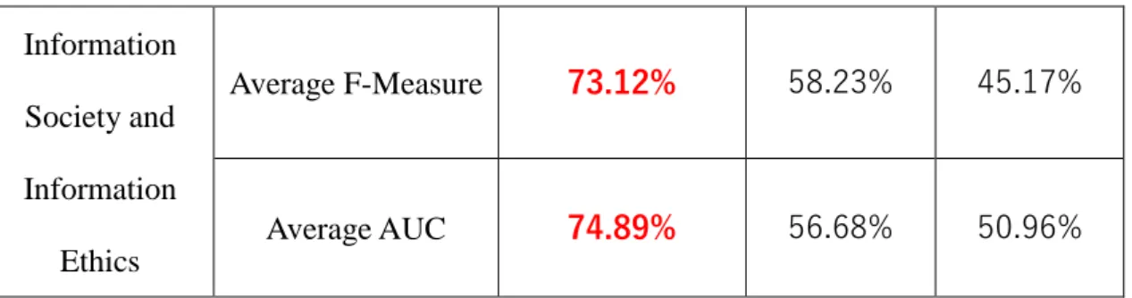
19 Information Society and Information Ethics Average F-Measure 73.12% 58.23% 45.17% Average AUC 74.89% 56.68% 50.96% 0 0.2 0.4 0.6 0.8 1 1 2 3 4 5 6 7 Re spo nse pr ed ic tion A cc urac y Task number Proposed Model HMIRT Model IRT Model
Fig. 6 Prediction accuracy of Foundation of Programming 1 (7 tasks, 148 learners).
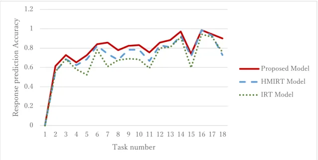
20 0 0.2 0.4 0.6 0.8 1 1.2 1 2 3 4 5 6 7 8 9 10 11 12 13 14 15 16 17 18 Re spo nse pr ed ic tion A cc urac y Task number Proposed Model HMIRT Model IRT Model 0 0.2 0.4 0.6 0.8 1 1 2 3 4 5 6 7 8 9 10 11 12 13 Re spo nse p red ic tion A cc urac y Task number Proposed Model HMIRT Model IRT Model
Fig. 7 Prediction accuracy of Foundation of Programming 2 (18 tasks, 77 learners).
Fig. 8 Prediction accuracy of Information Society and Information Ethics (13 tasks, 23 learners).
21
6.2. Window Size Parameter
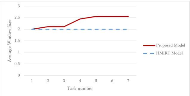
Figures 9–11 show how the window size changed during the learning process. Fig. 9
shows that for the Foundation of Programming 1 dataset, the window size tended to change only a small amount in the early time states, with larger changes later on. This can
be related to the response prediction accuracy in Fig. 6, where the response prediction accuracy of the proposed model only changes slightly compared with the response
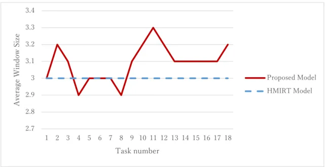
prediction accuracy of the HMIRT model in the first 3 tasks. Fig. 10 clearly shows the changes in the window size parameter for each item in the Foundation of Programming 2
dataset. The response prediction accuracy of this dataset (Fig. 7) also shows that the proposed model has a better response prediction accuracy. However, in Fig. 11, where the
size of the Information Society and Information Ethics dataset is small, the window size does not change for any time state.
0 0.5 1 1.5 2 2.5 3 1 2 3 4 5 6 7 A ve rag e W ind o w S iz e Task number Proposed Model HMIRT Model
Fig. 9 Window size of Foundation of Programming 1 (7 tasks, 148 learners).
22 1 1.5 2 2.5 3 1 2 3 4 5 6 7 8 9 10 11 12 13 A ve rag e W ind o w S iz e Task number Proposed Model HMIRT Model 2.7 2.8 2.9 3 3.1 3.2 3.3 3.4 1 2 3 4 5 6 7 8 9 10 11 12 13 14 15 16 17 18 A ve rag e W ind o w S iz e Task number Proposed Model HMIRT Model
Fig. 10 Window size of Foundation of Programming 2 (18 tasks, 77 learners).
Fig. 11 Window size of Information Society and Information Ethics (13 tasks, 23 learners).
23
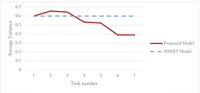
6.3. Variance Parameter
Figures 12–14 show how the variance parameter was set for each item. Fig. 12 shows that
the variance begins high, then gradually decreases. This means that for the Foundation of Programming 1 dataset, the learner’s ability will likely change by some large amount at first, then as the learning progresses, the changes in the learner’s ability will be smaller.
In Fig. 13, showing the Foundation of Programming 2 dataset, the variance of the
proposed model starts off quite low, then increases as the learning progresses. The variance peaks at item 11, then starts to fall until the end of the learning process. In Fig.
14, representing the Information Society and Information Ethics dataset where the dataset size is small, the variance of the proposed model is exactly the same as that of the HMIRT
model from the beginning to item 10. This can be related to the predictions of this dataset (Fig. 8), as the predictions of the proposed model are exactly the same as those of the
HMIRT model from the beginning until item 10. However, from item 11 onward, by decreasing the variance, the response prediction accuracy of the proposed model is now
better than that of HMIRT.
0 0.1 0.2 0.3 0.4 0.5 0.6 0.7 1 2 3 4 5 6 7 A ve rag e V aria nc e Task number Proposed Model HMIRT Model
Fig. 12 Variance of Foundation of Programming 1 (7 tasks, 148 learners).
24 0 0.2 0.4 0.6 0.8 1 1.2 1 2 3 4 5 6 7 8 9 10 11 12 13 A ve rag e V aria nc e Task number Proposed Model HMIRT Model 0 0.1 0.2 0.3 0.4 0.5 0.6 0.7 1 2 3 4 5 6 7 8 9 10 11 12 13 14 15 16 17 18 A ve rag e V aria nc e Task number Proposed Model HMIRT Model
Fig. 13 Variance of Foundation of Programming 2 (18 tasks, 77 learners).
Fig. 14 Variance of Information Society and Information Ethics (13 tasks, 23 learners).
25
7. Conclusion
In this research, we proposed a new method to estimate the learner’s ability from the
learning data, then used the estimated ability to predict the response for future tasks. The proposed model, AFHMIRT, generalizes the Hidden Markov Item Response Theory and
replaces the fixed values of the window size and variance parameters with time-series so that the parameters can fluctuate as learning progresses. In addition, we also proposed
using a linear search algorithm to estimate the window size parameter. From the results of the experiment, we demonstrated that modeling the window size and variance
parameters as time-series rather than fixed values resulted in a better response prediction accuracy. Moreover, the responses were predicted by the proposed model for one item at
a time, whereas the HMIRT model predicts the responses for all items at once. This made the proposed model’s predictions more precise. However, the proposed model has a
disadvantage with respect to estimation time. As described in Section 4, the proposed model needs to re-estimate the item parameter for all possible window size or the
variances to obtain the optimal value, which requires a lot of time to run, especially for larger datasets. Improving the estimation time will be considered in future tasks.
26
8. Reference
[1] L.S. Vygotsky, Thought and language,Harvard University Press,1962.
[2] L.S. Vygotsky, Mind in society,Harvard University Press,1978.
[3] D.Wood, J.S.Bruner, and G.Ross, ” The role of tutoring in problem solving.” ,Journal
of child psychiatry and psychology, and allied disciplines, pp.89-100,1976.
[4] A.Collins, "JS & Newman,SE(1989).Cognitive apprenticeship: teaching the craft of
reading, writing and mathematics,” Resnick, LB Knowing, learning and instruction, pp.453–494, 1989.
[5] J.Bruner, The Culture of Education, Harvard University Press, 1996, 1996.
[6] 植野真臣, 松尾淳哉, "項目反応理論を用いて適応的ヒントを提示する足場 かけシステム", 電子情報通信学会論文誌 D, Vol.J98-D,No.1,pp.17-29,Jan.2015. [7] M. Ueno, and Y. Miyazawa, "Probability based scaffolding system with fading",
Artificial Intelligencein Education - 17th International Conference, AIED 2015. pp.492-503,2015.
[8] M. Ueno, Y. Miyazawa: IRT-Based Adaptive Hints to Scaffold Learning in Programming, IEEE Transactions on Learning Technologies, IEEE computer Society,
Vol.11, Issue 4, 415-428 (2018)
[9] Baker,B,F, and Kim,S.: Item Response Theory: Parameter Estimation Techniques,
Second Edition, NY:Marcel Dekker, Inc,2004(2004)
[10] E. Tsutsumi, M. Uto,M. Ueno: "Bayesian Knowledge Tracing の一般化としての 隠れマルコフ IRT モデル",人工知能学会 2019 年度人工知能学会全国大会(第 33 回),2019
[11] 堤 瑛美子,宇都 雅輝,植野 真臣.”時系列学習データを用いた隠れマルコ フ IRT による高精度パフォーマンス予測”,日本行動計量学会 第 47 回大会,2019 [12] F.M. Lord, Applications of item response theory to practical testing problems,
27
Mahwah, NJ: Lawrence Erlbaum Associates, Inc,1980.
[13] S.Impedovo, A. Ferrante and R Modugno,"HMM Based Handwritten Word Recognition System by Using Singularities," Document Analysis and Recognition, 2009. ICDAR ’09. 10th International Conference on,2009.
[14] J.Ortiz, A.G.Olaya and D. Borrajo,"A Dynamic Sliding Window Approach for Activity Recognition"UMAP’11 Proceedings of the 19th international conference on
User modeling, adaption, and personalization,pp.219-230,2011.
[15] M. Ueno, "Data mining and text mining technologies for collaborative learning in an ILMS Samurai", Proc. IEEE Int. Conf. Adv. Learning Technol., pp. 1052-1053, 2004.