On the topology of the complements of quartic and
line configurations
Kenta Yoshizaki
(Received February 7, 2008)
Abstract. For a reduced plane curve C and a line L in P2, we put C2
L:= P2−L,
and CL:= C − (C ∩ L). If C and L intersect transversaly and π1(P2− C, b0) is abelian, it is known that π1(C2L− CL) is also abelian. In this article, we study
π1(C2L− CL) and the Alexander polynomial for the case when a quartic curve
C and a line L do not intersect transversaly.
AMS 2000 Mathematics Subject Classification. 14H20, 14H30. Key words and phrases. Fundamental group, Alexander polynomial.
§1. Introduction
Let C be a reduced plane curve in P2. We choose a line L ⊂ P2 and we put C2
L:= P2− L, and CL:= C − (C ∩ L). The line L is said to be generic with
respect to C if L intersects C transversaly.
L1 L2 L1:generic L2:non-generic C L3 L3:non-generic Figure 1.1
An element ω ∈ π1(P2− L, b0) is called a lasso for L if it is represented by a loop l ◦ τ ◦ l−1 where τ is a counter-clockwise oriented boundary of a small
disc D(p) of L at a point p ∈ L and l is a path connecting b0 and τ . In [O1], Oka proved the following:
Proposition 1.1 ([O1]) Let ω be a lasso for L and N (ω) be the subgroup normally generated by ω. Then the following sequence is exact:
1 → N (ω) → π1(C2L− CL) → π1(P2− C) → 1.
Moreover, if L is generic with respect to C, then
• ω is in the center of π1(C2L− CL) and N (ω) ∼= Z, and
• the equality D(π1(C2
L−CL)) = D(π1(P2−C)) holds, where D(?) denotes the commutator group of a group ?.
Note that we assume a base point b0 is chosen suitably. In the following, we omit the base points unless we need it explicitly.
By Proposition 1.1, when L is generic with respect to C, then π1(P2− C) is abelian if and only if π1(C2L− CL) is abelian. On the other hand, for a
non-generic line L, π1(C2L− CL) may be non-abelian. For example, when C is the
quartic defined by {X3Z + Y4= 0} which has an e6 singurality (= (3, 4)-cusp) at [0 : 0 : 1], and L∞ = {Z = 0} is the tangent line with multiplicity 4 at
[1:0:0], a presentation of the fundamental group π1(C2L− CL) is given by
π1(C2L− CL) ∼= ha, b, c | (abca)a = b(abca), c(abca) = (abca)b i
and its Alexander polynomial is
∆C(t, L) = (t2− t + 1)(t4− t2+ 1).
Hence π1(P2− C) ∼= Z/4Z, while π1(C2L− CL) is non-abelian. More such
examples can be found in [O3].
No. Singularities L∞ No. Singularities L∞
(1) 2a2 (i) (11) e6 (i) (2) 2a2 (iv) (12) e6 (iv) (3) 2a2+ a1 (i) (13) a3+ a2+ a1 (ii), a3 (4) 2a2+ a1 (iv) (14) a5+ a1 (i) (5) 3a2 (i) (15) a4+ a2 (ii), a2 (6) a2+ a3 (ii), a3 (16) a5+ a2 (iii), a2, a5 (7) a5 (i) (17) 2a3 (iii), 2a3 (8) a5 (iv) (18) a7 (v), a7 (9) a6 (ii), a6 (19) 2a3+ a1 (iii), 2a3 (10) a4+ a2 (v), a4 Table 1
Our purpose of this article is to study such phenomena for the case when C is a quartic and L is a non-generic line. For simplicity, we call such a configu-ration a QL-configuconfigu-ration. In [T], Tokunaga gave a list of QL-configuconfigu-rations which can be the branch loci of D2p-covers, where D2pis the dihedral group of order 2p with p an odd prime number. In particular, the fundamental groups of the complements of such configurations are non-abelian. In this article, we
give explicit models for QL-configurations in [T], presentations of π1(C2 L−CL)
and the Alexander polynomials of them. We remark that all intersection points of C and L are not transversal by [T, Corollary 3.5].
We introduce some notations in order to state our results. By a suitable projective transformation, we may regard L as the line at infinity L∞.
Thus we only have to study the fundamental group π1(C2− Ca), where Ca denotes the affine part of C which is defined by Ca:= C − (C ∩ L
∞). Table 1
is the list of the possible QL-configurations given in [T].
The numbers (i),. . .,(v) in the column of L∞ explain how C intersects L∞
as follows:
(i) L∞is bi-tangent to C at two distinct smooth points.
(ii) L∞is tangent to a smooth point and passes through a singular point of
C.
(iii) L∞passes through two distinct singular points.
(iv) L∞is tangent to C at a smooth point with intersection multiplicity 4.
(v) L∞intersects C at a singular point with intersection multiplicity 4. For notations for singularities, we use those in [M-P]. We first give an explicit model for each QL-configuration in Table 1. Note that L = L∞ and quartics
whose affine parts Ca are given by f (x, y) = 0 in Table 2. Here we put
x = X/Z, y = Y /Z. No. f (x, y) (1) −6 y3+ x4− 8 x2+ 16 − 2 y2x2+ 8 y2+ y4 (2) −y3+ x4− 2 x2+ 1 (3) 27 4 y 4− 16 y3+ 12 y2− 3 y + 1 4 − 27 2 x 2y2+27 4 x 4 (4) 16 9 x3− 2 x2− 6 x + 15 2 − 6 y2x − 9 y2− 1 2y4 (5) 18x2+ 18y2+ 24xy2− 8x3+ 2x2y2+ y4+ x4− 27 (6) 1 + 3 y − 4 y2x2+ 3 y2− 4 y3x + y3− y4 (7) 36 x4− 33 x3+ 10 x2− x − 12 y2x2+ 10 y2x − 2 y2+ y4 (8) −x3+ x2− 2 xy2+ y4 (9) 1 − 2 xy − 4 y + y2x2+ 4 xy2+ 6 y2− 2 xy3− 3 y3+ y4 (10) x3−¡x2− y + 1¢2 (11) (x − 1)3+ y4 (12) x3+ (y − x)2(y + x)2
(13) y¡81 x + 54 + 81 yx2− 54 yx − 54 y + 90 y2x + 18 y2+ 25 y3¢ (14) ¡y2− 2 yx − x + x2¢ ¡y2+ 2 yx − x + x2¢ (15) 256 y4− 256 y3+ 96 y2− 16 y + 1 + 32 xy3− 32 xy2+ 10 xy − x + x2y2 (16) (y − x)¡−y2x + 1 + y3¢ (17) ¡y2+ yx + 2¢ ¡y2+ yx + 1¢ (18) ¡−x − 2 + y2¢ ¡−x − 1 + y2¢ (19) (−2 y + 1 + 2 x) (2 y + 1 + 2 x)¡−y2+ x2+ x¢ Table 2: Defining equations of Q Now we are ready to state our result.
Theorem 1.2 For the QL-configurations given by the quartic polynomials as above and L∞, we have presentations of the fundamental groups π1(C2L− CL)
and Alexander polynomials ∆C(t, L) as follows:
No. presentation of π1(C2L− CL) ∆C(t, L)
(1) ha, b | aba = babi t2− t + 1
(2) ha, b | aba = babi t2− t + 1
(3) ha, b | aba = babi t2− t + 1
(4) ha, b, c | aca = cac, cbc = bcb, ab = bai t2− t + 1 (5) ha, b, c | aba = bab, bcb = cbc, (t2− t + 1)2
c (b−1ab) c = (b−1ab) c (b−1ab)i
(6) ha, b | aba = babi t2− t + 1
(7) ha, b | aba = babi t2− t + 1
(8) ha, b | aba = babi t2− t + 1
(9) ha, b | aba = babi t2− t + 1
(10) ha, b | aba = babi t2− t + 1
(11) ha, b | aba = babi t2− t + 1
(12) ha, b, c | b(acba) = (acba)a, c(acba) = (acba)bi (t2− t + 1)(t4− t2+ 1) (13) ha, b, c | bcb = cbc, ac = ba, accb = cbaci (t − 1)(t2− t + 1) (14) ha, b | (ab)3 = (ba)3, babba = abbabi (t − 1)(t2− t + 1) (15) ha, b | ababa = babab, abb = bbai 1
(16) ha, b | bba = abbi t2− 1
(17) ha, b, c | ab = bci 1
(18) ha, b, c | ab = bci 1
(19) ha, b, c | bc = cb, bac = cabi (t − 1)2(t + 1) Table 3
Remark. Some Alexander polynomials in the above list are computed in [O3] by two ways. They are mainly obtained by the line degeneration method and
some are done by the Fox calculus. And the group represented by ha, b | aba = babi is isomorphic to the braid group B3 of 3 strings.
§2. Preliminaries 2.1. Zariski-van Kampen’s method
In this subsection, we briefly summarize Zariski-van Kampen’s method in computing the fundamental group. For details, see [O3], [S] and [T-S]. Let Ca
be a reduced affine curve defined by a polynomial f (x, y) of degree d. By a suitable linear transformation of coordinate system, we may assume that the coefficient of yd is a non-zero constant.
Let p : C2 − Ca → C be a map given by (x, y) 7→ x. For s ∈ C,
y-coordinates of the intersection points of the affine line {x = s} and C are corresponding to roots of the equation f (s, y) = 0. We denote by D(f,y)(s) the discriminant with respect to y and put
Σ := {s ∈ C | D(f,y)(s) = 0}.
We call lines {x = s | s ∈ Σ} singular lines. Since Ca is reduced, Σ is a finite set. For all t ∈ C − Σ, p−1(t) is isomorphic to the d-punctured affine line and
restriction
p|p−1(C−Σ) : p−1(C − Σ) → C − Σ
is the local trivial fibration.
We choose a sufficiently large positive real number S such that a disc BS:=
{s ∈ C | |s| < S} contains Σ. Since the inclusion p−1(B
S) ,→ C2 − C gives
a homotopy equivalence, we only have to compute π1(p−1(BS)). Since the
coefficients of yd−ν, (ν > 0) in f (x, y) are polynomials in x and they are
bounded on BS, we can take a base point b0
0 = (b0, ˜b0) ∈ C2 − Ca where p(b00) = b0, b0∈ BS and (BS× { ˜b0}) ∩ C = ∅.
In this setting, the restriction of p p|p−1(B
S): p
−1(B
S) → BS
has the holomorphic section s 7→ (s, ˜b0) which passes through b00. Using this section, one can define an action of π1(BS − Σ, b0) on π1(p−1(b0), b00). We call this action the monodromy action. Let r be a number of points of Σ. Then π1(BS− Σ, b0) is the free group generated by loops γ1, γ2, . . . , γr, and
π1(p−1(b0), b00) is generated by loops g1, g2, . . . , gd. We denote the action of γj
on gi by gγj
Theorem 2.1 ([T-S], [S]) The inclusion map p−1(b
0) ,→ C2 − Ca induces an isomorphism
π1(p−1(b0), b00)/N → π1(C2− Ca, b00),
where N is the minimal normal subgroup of π1(p−1(b0), b00) which contains {g−1i gγj
i | i = 1, 2, . . . , d, j = 1, 2, . . . , r}.
Thus the presentation of π1(C2− Ca, b00) is
hg1, g2, . . . , gd | gi= giγji i=1,2,...,d, j=1,2,...,r.
In particular, we call relations gi= giγj monodromy relations.
2.2. Some basic monodromy actions
In this subsection, we recall some basic monodromy actions. We consider curves whose local equations at (0, 0) given by
(i) h1 = x − y2, (ii) h2= x2− y2, (iii) h3= x3− y2.
Since the line x = 0 is a singular line for all cases, we take a base point x = ² and its general fiber F²= p−1(²), where ² is a sufficiently small positive
number. Since each hi have degree 2 with respect to y, F² is isomorphic to
the 2-punctured plane. We take meridians g1 and g2 as generators of π1(F²) as follows: F² F² F² g1 g2 F²= p−1(²) |x| = ² |x| = ² |x| = ² Figure 2.1
When x goes with counter clockwise direction along the circle |x| = ² which is the generator of π1(C − {0}), g1 and g2 are moved as following figures by the monodromy action.
g2 g1 g1 g2
g2 g1
(i) (ii) (iii)
Figure 2.2
By Theorem 2.1, we have monodromy relations of each cases: (i) g1 = g2 (ii) g1g2 = g2g1 (iii) g1g2g1= g2g1g2.
We call these relations the tangential relation, the nodal relation and the cus-pidal relation respectively.
2.3. Alexander polynomial
In this subsection, we briefly summarize Fox calculus in computing the Alexan-der polynomial. For details, see [C-F, 119p]. Suppose that G := π1(C2−Ca, b00) is given by the following finite representation:
G = hg1, . . . , gn | R1, . . . , Rmi,
where gi are generators of π1(p−1(b0)) and Ri denotes the monodromy
rela-tions. Let F (n) be a free group of rank = n which is generated by g1, . . . , gn.
Moreover we consider the group ring C£F (n)¤of F (n) with C-coefficient. The Fox differentials ∂g∂i : C£F (n)¤ → C£F (n)¤ are a C-linear operator which satisfies the following two properties:
(i) ∂ ∂gj(gi) = δij, (ii) ∂ ∂gj(uv) = ∂u ∂gj + u ∂v ∂gj, u, v ∈ C [F (n)] .
Let γ : C [F (n)] → C[t, t−1] be a ring homomorphism defined by g
i, g−1i 7−→
t, t−1 for all i. Now we get (m × n)-matrix whose elements are in C[t, t−1]. We put A := Ã γ µ ∂Ri ∂gj ¶!
and call A the Alexander matrix. Then Alexander polynomial ∆C(t) is given
by the greatest common divisor of the determinants of all (n − 1) × (n − 1) submatrices of the Alexander matrix A if m ≥ n − 1, and it is understood that
∆C(t) = 0 if n − 1 > m,
Example 2.2 For the group presentad by ha, b | aba = babi, we put the mon-odromy relation as R = abab−1a−1b−1. Then we have
∂R
∂a = 1 + ab − abab
−1a−1, ∂R
∂b = a − abab
−1− abab−1a−1b−1.
Moreover the Alexander matrix A and Alexander polynomial ∆(t) are given as follows.
A =£ 1 + t2− t t − t2− 1 ¤, ∆(t) = t2− t + 1.
§3. Proof of Theorem 1.2
In this section, we give a proof of Theorem 1.2. Since our proof is done by case by case computation and most of them are similar, we give complete proofs for the cases (5) and (9), and rough sketches for the remaining cases.
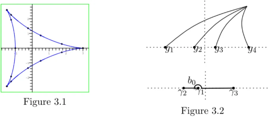
Case (5): In this case, Q is a quartic with 3a2 and L is its unique bi-tangent line. As we have seen in the introduction, such an example is given by an equation
F (X, Y, Z) := 18X2Z2+18Y2Z2+24XY2Z−8X3Z+2X2Y2+Y4+X4−27Z4. When we put C = {F (X, Y, Z) = 0} and its affine part Ca = {f (x, y) =
F (x, y, 1) = 0}, then
(i) C has three cusps at [3 : 0 : 1] and [−3/2 : ±3√3/2 : 1], (ii) L∞= {Z = 0} is bi-tangent to C, and
(iii) the discriminant of f with respect to y is
4096(x + 1)(x − 3)3(2x + 3)6.
Figure 3.1 shows the graph of the real part of Ca. Put Σ = {x ∈ C | x =
−3/2, −1, 3} and take the base point b0 := −1 − ², where ² is a small positive real number. We denote by F0 the fiber p−1(b
0) which is isomorphic to 4-punctured plane. 2 1 -1 -1 3 1 2 -2 0 0 Figure 3.1 g1 g2 g3 g4 γ2 γ1 γ3 b0 Figure 3.2
To compute the monodromy action by the fundamental group of base space π1(C − Σ, b0), we fix g1, g2, g3, g4 as generators of π1(F0, b00), and meridians γ1, γ2, γ3 as generators of π1(C − Σ, b0), where γ1, γ2 and γ3 are given by the following:
• γ1: the meridian of x = −1 from b0 • γ2: the meridian of x = −3/2 from b0
• γ3: the meridian of x = 3 from b0 stepping aside x = −1.
Figure 3.2 shows our choice of g1, g2, g3, g4 and γ1, γ2, γ3. Note that • denotes a circle. In this setting, we see each monodromy actions explicitly.
Monodromy action of γ1: Since g2 and g3 have the tangential relation, we obtain g2 = g3.
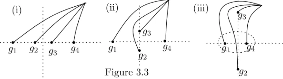
Monodromy action of γ2: Since g1, g2and g3, g4have the cuspidal relations each other, we obtain g1g2g1= g2g1g2 and g3g4g3 = g4g3g4.
g1 g2 g3 g4 g1 g4 g3 g2 g3 g2 g4 g1
(i) (ii) (iii)
Figure 3.3
Monodromy action of γ3: Figure 3.3 corresponds each steps of the monodromy action with respect to γ2 as follows:
(i) start position,
(ii) z comes close to −1 and steps aside −1, (iii) z comes close to 3.
By Figure 3.3, we can observe g1 and g4 have the cuspidal relation.
g2 h1 g4 h3 g2 g4 g1 g3 Figure 3.4
For simplicity, we replace two generators g1 and g3 by h1 and h3 as in Figure 3.4. Namely we put
h1 = g2−1g1g2, h3= g1g3g1−1.
h1 and g4 have the cuspidal relation, we just only obtain g4h1g4= h1g4h1. By Theorem 2.1,
π1(C2
L− CL) ∼= hg1, g2, g4, h1 | g1g2g1 = g2g1g2, g2g4g2 = g4g2g4, g4h1g4= h1g4h1, h1= g2−1g1g2i.
Now the Alexander matrix A and its Alexander polynomial are A = t 2− t + 1 −t2+ t − 1 0 0 t2− t + 1 −t2+ t − 1 t − t2+ 1 (1 − t)(t2− t + 1) t2− t + 1 , ∆C(t) = (t2− t + 1)2.
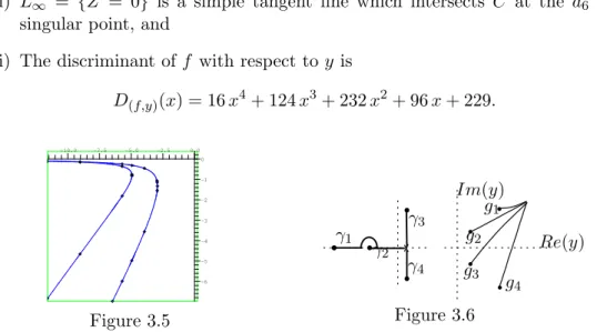
Case (9): In this case, Q is a quartic with an a6 singularity and L is its unique tangent line which intersects C at the a6 singular point. As we have seen in the introduction, such an example is given by an equation
F := X4−2 Z2Y X −4 Z3Y +Y2X2+4 ZY2X +6 Y2Z2−2 XY3−3 ZY3+Y4. When we put C = {F (X, Y, Z) = 0} and its affine part Ca = {f (x, y) =
F (x, y, 1) = 0}, then
(i) C has an a6 singularity at [1 : 0 : 0],
(ii) L∞ = {Z = 0} is a simple tangent line which intersects C at the a6 singular point, and
(iii) The discriminant of f with respect to y is
D(f,y)(x) = 16 x4+ 124 x3+ 232 x2+ 96 x + 229. 0.0 -5 0 -1 -2 -10.0 -5.0 -6 -3 -2.5 -7.5 -4 Figure 3.5 Re(y) Im(y) g1 g2 g3 g4 γ1 γ2 γ4 γ3 Figure 3.6
Figure 3.5 shows the graph of the real part of Ca. We put Σ := {α1, α2, β, β}, where αiare real roots of D(f,y)(x) = 0 and β, β are complex roots. We assume that α1 < α2. Take the base point b0 of C − Σ at b0 = Re(β) = Re(β) ∈ C
and meridians γ1, γ2, γ3, γ4 as generators of π1(C − Σ, b0). For F0 = p−1(b 0), we also fix meridians g1, g2, g3, g4 as generators of π1(F0, b00). Figure 3.6 shows our setting of generators.
Monodromy action of γ3: By Figure 3.7, we have g2 = g4 immediately. Similarly, we have monodromy relation g1= g3 with γ4.
g1 g2 g4 g3 b0 β Figure 3.7 g1 g2 g3 g4 b0 α2 Figure 3.8
Monodromy action of γ2: By Figure 3.8, g1and g4 have the tangential rela-tion. Considering the homotopy equivarence of roops, we have the monodromy relation,
g1g2g3 = g2g3g4.
By using previous relations g2= g4 and g1 = g3, this relation implies g1g2g1 = g2g1g2. g1 g2 g3 g 4 h1 h2 h3 h 4 Figure 3.9
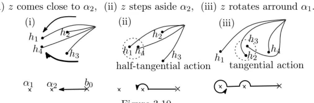
Monodromy action of γ1: For simplicity, we replace generators as follows: h1= g1, h2= g2, h3= g3, h4= g3g4g3−1.
Figure 3.9 explains how to replace the base position of generators, and Figure 3.10 corresponds each steps of the monodromy action with respect to γ1:
(i) z comes close to α2, (ii) z steps aside α2, (iii) z rotates arround α1.
α1 α2 b0
half-tangential action tangential action h1 h4 h2 h3 h2 h3 h4 h1 h 1 h4 h3 h2 Figure 3.10
(i) (ii) (iii)
By Figure 3.10, we have just one monodromy relation with γ1: h2= h4h3h−14 ⇔ h2h4= h4h3.
Rewriting this relation into g1, g2, g3, g4, and g1= g3, g2 = g4, we obtain g2g1g2 = g1g2g1.
By Theorem 2.1, we have
π1(C2L− CL) ∼= hg1, g2 | g2g1g2= g1g2g1i.
Moreover the Alexander polynomial is equal to t2− t + 1 by Example 2.2. For simplicity, we sometimes denote the monodromy action of each γi and
its monodromy relations by γi-action and γi-relation in the following sketch of proofs.
Case (1): We consider the following homogenized polynomial:
F (X, Y, Z) := 16 Z4− 8 X2Z2+ X4+ 8 Y2Z2− 2 Y2X2− 6 Y3Z + Y4. When we put C = {F (X, Y, Z) = 0} and its affine part Ca = {f (x, y) =
F (x, y, 1) = 0}, then
(i) C has two cusps at [±2 : 0 : 1] ,
(ii) L∞= {Z = 0} is a bi-tangent line, and
(iii) the discriminant of f with respect to y is
D(f,y)(x) = −144 (x − 2)4(x + 2)4¡64 x2− 13¢.
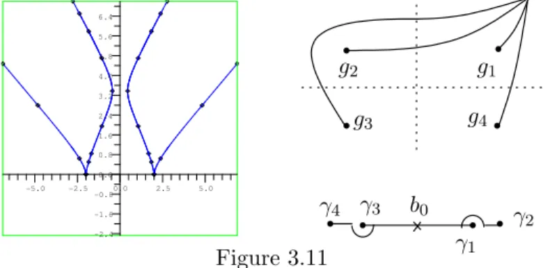
Figure 3.11 shows the real part of the affine curve Ca and the setting of
generators. 5.6 4.0 0.8 4.8 -1.6 0.0 -5.0 2.5 0.0 -0.8 1.6 5.0 -2.4 2.4 6.4 -2.5 3.2 g1 g2 g3 g4 b0 γ1 γ2 γ3 γ4 Figure 3.11
Put Σ := {x ∈ C | D(f,y)(x) = 0} and take a base point b0 = 0 ∈ C − Σ. Furthermore, we take generators of π1(C − Σ, b0) and π1(p−1(b0), b00) as Figure 3.12. Monodromy relations with each γi are
Since f (x, y) = f (−x, y), monodromy relations with γ3 and γ4 are same to γ1-relation and γ2-relation. By Theorem 2.1 and Example 2.2, we have
π1(C2L− CL) ∼= hg1, g2 | g1g2g1 = g2g1g2i, ∆C(t, L) = t2− t + 1.
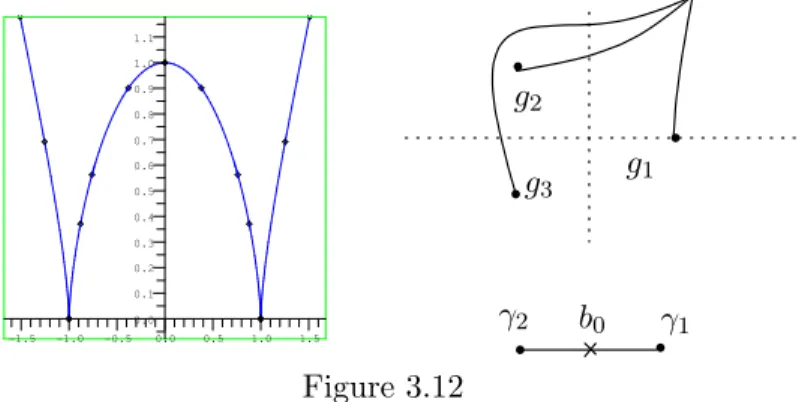
Case (2): We consider the following homogenized polynomial: F (X, Y, Z) := −Y3Z + X4− 2 X2Z2+ Z4.
When we put C = {F (X, Y, Z) = 0} and its affine part Ca = {f (x, y) =
F (x, y, 1) = 0}, then
(i) C has two cusps at [±1 : 0 : 1] ,
(ii) L∞= {Z = 0} is a tangent line with multiplicity 4, and (iii) the discriminant of f with respect to y is
D(f,y)(x) = −27 (x − 1)4(x + 1)4.
Figure 3.12 show the real part of the affine curve Ca and the setting of
gener-ators. 1.0 -1.0 1.5 1.1 0.9 0.0 0.6 0.4 0.5 0.1 -0.5 -1.5 0.7 0.0 0.5 1.0 0.2 0.3 0.8 g1 g2 g3 b0 γ1 γ2 Figure 3.12
Put Σ := {x ∈ C | D(f,y)(x) = 0} and take a base point b0 = 0 ∈ C − Σ. Moreover, we take generators of π1(C − Σ, b0) and π1(p−1(b0), b00) as Figure 3.13. Monodromy relations with γ1 are
g1 = g3, g1g2g1 = g2g1g2.
Since f (x, y) = f (−x, y), the monodromy relation with γ2 is same to the γ1 -relation. By Theorem 2.1 and Example 2.2, we have
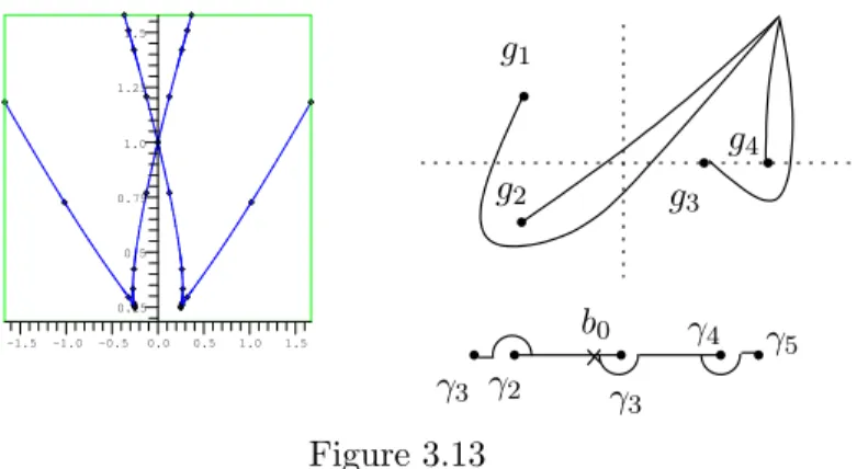
Case (3): We consider the following homogenized polynomial: F (X, Y, Z) := 27 4 Y 4− 16 Y3Z + 12 Y2Z2− 3 Y Z3+1 4Z 4−27 2 X 2Y2+27 4 X 4. When we put C = {F (X, Y, Z) = 0} and its affine part Ca = {f (x, y) =
F (x, y, 1) = 0}, then
(i) C has two cusps and a1 singular point at [±1/4 : 1/4 : 1], [0 : 1 : 1] respectively,
(ii) L∞= {Z = 0} is a bi-tangent line, and
(iii) the discriminant of f with respect to y is D(f,y)(x) = −19683
16 x
2¡27x2− 2¢(4x − 1)3(4x + 1)3.
Figure 3.13 shows the real part of the affine curve Ca and the setting of
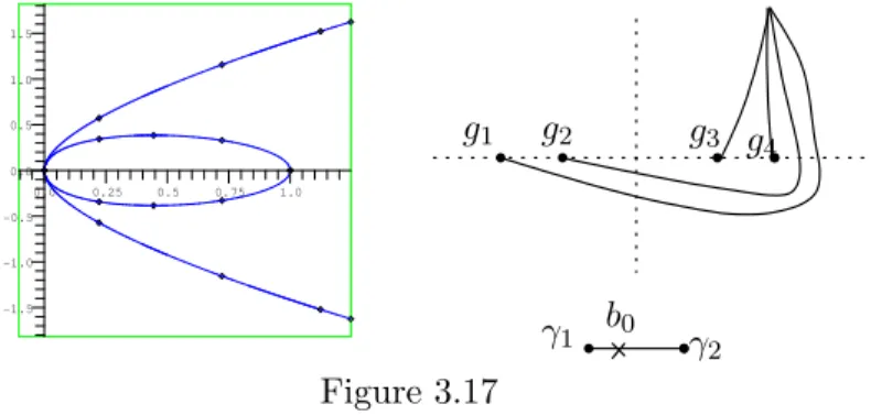
generators. 1.5 1.0 0.5 0.0 -0.5 0.25 0.75 1.0 -1.0 1.25 -1.5 1.5 0.5 g1 g2 g3 g4 b0 γ5 γ3 γ2 γ3 γ4 Figure 3.13
Put Σ := {x ∈ C | D(f,y)(x) = 0} and take a base point b0 = −² ∈ C − Σ, where ² is a sufficiently small positive real number. Moreover, we take generators of π1(C − Σ, b0) and π1(p−1(b0), b00) as Figure 3.14. Monodromy relations with each γi are
(γ1) g3g4 = g4g3, (γ2) g1g2g1= g2g1g2, (γ3) g1 = g4g3g−14 , (γ5) g1 = g4.
Since f (x, y) = f (−x, y), γ4-action is same to γ2-action. By Theorem 2.1 and Example 2.2, we have
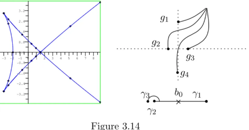
Case (4): We consider the following homogenized polynomial: F (X, Y, Z) := 16 9 X 3Z − 2X2Z2− 6XZ3+15 2 Z 4− 6XY2Z − 9Y2Z2−1 2Y 4. When we put C = {F (X, Y, Z) = 0} and its affine part Ca = {f (x, y) =
F (x, y, 1) = 0}, then
(i) C has two cusps and an a1 singular point at [−3 : ±3 : 1], [3/2 : 0 : 1], (ii) L∞= {Z = 0} is a tangent line with multiplicity 4, and
(iii) the discriminant of f with respect to y is D(f,y)(x) = −4096
729 (8x + 15) (2x − 3)
2(x + 3)6.
Figure 3.14 shows the real part of the affine curve Ca and the setting of
generators. 8 7 6 5 4 3.2 -3 0.8 1 1.6 -3.2 -1.6 2.4 -2.4 -0.8 0 -1 3 0.0 -2 2 g1 g2 g3 g4 b0 γ3 γ1 γ2 Figure 3.14
Put Σ := {x ∈ C | D(f,y)(x) = 0} and take a base point b0 = 3/2 − ² ∈ C − Σ, where ² is a sufficiently small positive real number. We also take generators of π1(C − Σ, b0) and π1(p−1(b0), b00) as Figure 3.15. Monodromy relations with γi are
(γ1) g2g3 = g3g2, (γ2) g1 = g4, (γ3) g1g2g1= g2g1g2, g3g4g3= g4g3g4. By Theorem 2.1, we have
π1(C2L− CL) ∼= hg1, g2, g3 | g1g2g1= g2g1g2, g1g3g1= g3g1g3, g2g3= g3g2i. By this presentation, the Alexander matrix A and its Alexander polynomial are given by A = t 2− t + 1 −t2+ t − 1 0 t2− t + 1 0 −t2+ t − 1 0 1 − t t − 1 , ∆C(t, L) = t2− t + 1.
Case (6): We consider the following homogenized polynomial: F (X, Y, Z) := Z4+ 3Y Z3− 4X2Y2+ 3Y2Z2− 4XY3+ Y3Z − Y4. When we put C = {F (X, Y, Z) = 0} and its affine part Ca = {f (x, y) =
F (x, y, 1) = 0}, then
(i) C has one a3 and one a2 singular points at [1 : 0 : 0], [1/2, −1, 1] respec-tively,
(ii) L∞= {Z = 0} is a tangent line which passes through a3 , and (iii) the discriminant of f with respect to y is
D(f,y)(x) = −¡256x4− 32x3− 480x2+ 822x − 283¢(2x − 1)3. Figure 3.15 shows the real part of the affine curve Ca and the setting of generators. -1 -1 5 -2 7 1 4 0 1 8 0 3 2 6 g1 g2 g3 g4 b0 γ4 γ3 γ2 γ1 γ5 Figure 3.15
Put Σ := {x ∈ C | D(f,y)(x) = 0} and take a base point b0 = α ∈ C − Σ, where α is the real part of the complex root of 256 x4− 32 x3− 480 x2+ 822 x − 283 = 0. We take generators of π1(C − Σ, b0) and π1(p−1(b0), b00) as Figure 3.16. Monodromy relations with each γi are
(γ1) g1g2g1 = g2g1g2, (γ2) g1= g3, (γ3) g1 = g3, (γ4) g2= g3g4g3−1, (γ5) g4 = g2g1g−12 .
Computing these relations, we have g1g2g1 = g2g1g2. By Theorem 2.1 and Example 2.2, we have
Case (7): We consider the following homogenized polynomial:
F (X, Y, Z) := 36X4−33X3Z+10X2Y2−XZ3−12X2Y2+10XY2Z−2Y2Z2+Y4. When we put C = {F (X, Y, Z) = 0} and its affine part Ca = {f (x, y) =
F (x, y, 1) = 0}, then
(i) C has an a5 singular point at [1/3 : 0 : 1], (ii) L∞= {Z = 0} is a bi-tangent line, and (iii) the discriminant of f with respect to y is
D(f,y)(x) = 256x (4x − 1) (−1 + 3x)8.
The Figure 3.16 shows the real part of the affine curve Ca and the setting of
generators. 0.1 0.0 0.2 1.5 0.0 0.3 1.0 -1.0 -0.5 0.5 -1.5 g1 g2 g3 g4 b0 γ3 γ1 γ2 Figure 3.16
Put Σ := {x ∈ C | D(f,y)(x) = 0} and take a base point b0 = 1/3 − ² ∈ C − Σ, where ² is a sufficiently small positive real number. Moreover, we take generators of π1(C − Σ, b0) and π1(p−1(b0), b00) as Figure 3.17. Monodromy relations with each γi are
(γ1) g1 = g3, g2= g3g4g3−1, g4 = (g3g4g2g1)g2(g3g4g2g1)−1,
(γ2) g3 = g3g4g2(g3g4)−1.
Since the relative position of g1 and g4 about γ3 is fixed on real axis, the γ3-relation is same to that of γ2-relation. Computing these relations, we have g1g2g1 = g2g1g2. By Theorem 2.1 and Example 2.2, we have
π1(C2L− CL) ∼= hg1, g2 | g1g2g1 = g2g1g2i, ∆C(t, L) = t2− t + 1.
Case (8): We consider the following homogenized polynomial: F (X, Y, Z) := −X3Z + X2Z2− 2XY2Z + Y4.
When we put C = {F (X, Y, Z) = 0} and its affine part Ca = {f (x, y) =
(i) C has an a5 singular point at [0 : 0 : 1],
(ii) L∞= {Z = 0} is a tangent line with multiplicity 4, and
(iii) the discriminant of f with respect to y is D(f,y)(x) = −256x8(x − 1). Figure 3.17 shows the real part of the affine curve Ca and the setting of
generators. 0.75 0.25 -0.5 1.0 -1.0 0.0 1.5 0.0 1.0 0.5 0.5 -1.5 g1 g2 g3 g4 b0 γ1 γ2 Figure 3.17
Put Σ := {x ∈ C | D(f,y)(x) = 0} and take a base point b0 = ² ∈ C − Σ, where ² is a sufficiently small positive real number. We take generators of π1(C − Σ, b0) and π1(p−1(b0), b00) as Figure 3.17. Monodromy relations with each γi are
(γ1) g1 = g3, g2= g3g4g3−1, g4 = (g3g4g2g1)g2(g3g4g2g1)−1, (γ2) g3 = g3g4g2(g3g4)−1.
Computing these relations, we have g1g2g1 = g2g1g2. By Theorem 2.1 and Example 2.2, we have
π1(C2L− CL) ∼= hg1, g2 | g1g2g1 = g2g1g2i, ∆C(t, L) = t2− t + 1.
Case (10): We consider the following homogenized polynomial: F (X, Y, Z) := X3Z −¡X2− Y Z + Z2¢2.
When we put C = {F (X, Y, Z) = 0} and its affine part Ca = {f (x, y) = F (x, y, 1) = 0}, then
(i) C has one a4 and one a2 at [0 : 1 : 0], [0, 1, 1] respectively, (ii) L∞= {Z = 0} is a line which intersects at the a4 singular, and (iii) The discriminant of f with respect to y is D(f,y)(x) = 4x3.
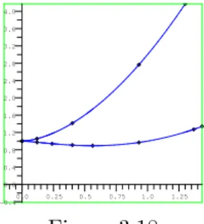
2.8 2.0 1.2 1.25 -0.4 4.0 3.6 3.2 2.4 1.6 0.8 0.4 0.0 1.0 0.75 0.5 0.0 0.25 Figure 3.18
Figure 3.18 shows the real part of the affine curve Ca. By the graph and
the discriminant with respect to y, we can clearly see that all monodromy relations are only one cuspidal relation. By Theorem 2.1 and Example 2.2, we have
π1(C2L− CL) ∼= hg1, g2 | g1g2g1= g2g1g2i, ∆C(t, L) = t2− t + 1.
Case (11): We consider the following homogenized polynomial: F (X, Y, Z) := X3Z + (Y − X)2(Y + X)2.
When we put C = {F (X, Y, Z) = 0} and its affine part Ca = {f (x, y) =
F (x, y, 1) = 0}, then
(i) C has an e6 singular point at [0 : 0 : 1], (ii) L∞= {Z = 0} is a bi-tangent line, and
(iii) the discriminant of f with respect to y is D(f,y)(x) = 256x9(1 + x) . Figure 3.19 shows the real part of the affine curve Ca and the setting of
generators. 1.2 0.8 -1.2 -2.0 -0.8 -1.0 1.6 0.0 -1.6 -0.5 -1.5 0.4 0.0 -0.4 g1 g2 g3 g4 b0 γ1 γ2 Figure 3.19
Put Σ := {x ∈ C | D(f,y)(x) = 0} and take a base point b0 = −1 + ² ∈ C − Σ, where ² is a small number. Moreover, we take generators of π1(C − Σ, b0) and
π1(p−1(b
0), b00) as Figure 3.19. Monodromy relations with each γi are
(γ1) g1= g4, g2 = (g4g3g2)g1(g4g3g2)−1, g3 = (g4g3g2g1)g2(g4g3g2g1)−1, (γ2) g2= (g3g2)−1g4(g3g2).
Computing these relations, we have g1g3g1 = g3g1g3. By Theorem 2.1 and Example 2.2, we have
π1(C2L− CL) ∼= hg1, g3 | g1g3g1 = g3g1g3i, ∆C(t, L) = t2− t + 1.
Case (12): We consider the following homogenized polynomial: F (X, Y, Z) := (X − Z)3Z + Y4.
When we put C = {F (X, Y, Z) = 0} and its affine part Ca = {f (x, y) =
F (x, y, 1) = 0}, then
(i) C has an e6 singular point at [1 : 0 : 1],
(ii) L∞= {Z = 0} is a tangent line with multiplicity 4, and
(iii) The discriminant of f with respect to y is 256 (x − 1)9.
-0.2 -0.8 0.8 0.2 0.4 0.6 1.0 0.6 0.8 0.0 -0.6 0.2 -0.4 0.4 Figure 3.20
Figure 3.20 shows the real part of the affine curve Ca. As we can observe
clearly by the graph and the discriminant with respect to y, all monodromy relations are given by the e6-action of γ1. Monodromy relations are
g1= g4, g2 = (g4g3g2)g1(g4g3g2)−1, g3 = (g4g3g2g1)g2(g4g3g2g1)−1. Computing these relations and replacing w = g1g3g2g1. By Theorem 2.1, we have
hg1, g2, g3 | wg1 = g2w, wg2 = g3wi.
Then the Alexander matrix and the Alexander polynomial are given by A =
·
t − t3− 1 t3− t2+ 1 t(t − 1) t4− t3+ t − 1 −t2(t2− t + 1) t2− t + 1
∆C(t, L) = (t2− t + 1)(t4− t2+ 1).
Case (13): We consider the following homogenized polynomial: F (X, Y, Z) := Y (81XZ2+ 54Z4+ 81X2Y − 54XY Z − 54Y Z2
+ 90XY2+ 18Y2Z + 25Y3).
When we put C = {F (X, Y, Z) = 0} and its affine part Ca = {f (x, y) = F (x, y, 1) = 0}, then
(i) C has one a1, one a2 and one a3 sigular points at [−2/3 : 0 : 1], [−3/4 : 3/4 : 1], [1 : 0 : 0] respectively,
(ii) L∞ = {Z = 0} is a tangent line which intersects C at the a3 singular point, and
(iii) the discriminant of f with respect to y is
D(f,y)(x) = 243 (3x + 2)2¡5x2− 12x − 12¢(4x + 3)3.
Figure 3.21 shows the real part of the affine curve Ca and the setting of
generators. -7 -1 -4 -10 -1 -8 -11 1 0 -6 3 -9 -5 -2 0 1 -3 2 g1 g2 g3 g4 b0 γ4 γ1 γ2 γ3 Figure 3.21
Put Σ := {x ∈ C | D(f,y)(x) = 0} and take a base point b0= −3/4−² ∈ C−Σ, where ² is a sufficiently small positive real number. We take generators of π1(C − Σ, b0) and π1(p−1(b0), b00) as Figure 3.21. Monodromy relations with each γi are
(γ1) g4g3g4−1= g2, (γ2) g3g4g3 = g4g3g4, (γ3) g1g2 = g2g1, (γ4) g1g4 = g3g1. By Theorem 2.1, we have
Then the Alexander matrix and the Alexander polynomial are A = 0 t 2− t + 1 −t2+ t − 1 1 − t2 t(t2− 1) −t3+ t2+ t − 1 1 − t −1 t , ∆C(t, L) = (t2− t + 1)(t − 1).
Case (14): We consider the following homogenized polynomial: F (X, Y, Z) :=¡Y2− 2XY − XZ + X2¢ ¡Y2+ 2XY − XZ + X2¢. When we put C = {F (X, Y, Z) = 0} and its affine part Ca = {f (x, y) = F (x, y, 1) = 0}, then
(i) C has one a5 and one a1 singular points at [0 : 0 : 1], [1 : 0 : 1], (ii) L∞= {Z = 0} is a bi-tangent line, and
(iii) the discriminant of f with respect to y is
D(f,y)(x) = 4096x8(−1 + x)2.
Figure 3.22 shows the real part of the affine curve Ca and the setting of
generators. 2.0 1.6 1.2 0.8 0.0 -0.8 -1.6 -2.4 0.4 -0.4 -1.2 -2.0 1.5 1.0 1.25 0.5 2.4 0.0 0.25 0.75 g1 g2 g3 g4 b0 γ1 γ2 Figure 3.22
Put Σ := {x ∈ C | D(f,y)(x) = 0} and take a base point b0 = ² ∈ C − Σ, where ² is a sufficiently small positive real number. We also take generators of π1(C − Σ, b0) and π1(p−1(b
0), b00) as Figure 3.22. Monodromy relations with each γi are
(γ1) g1 = g3, g2= g3g4g3−1, g4 = (g3g4g2g1)g2(g3g4g2g1)−1, (γ2) g3g3g4g2(g3g4)−1= g
3g4g2(g3g4)−1g3.
Computing these relations, we have g2g1g2g2g1 = g1g2g2g1g2 and (g1g2)3 = (g2g1)3. By theorem 2.1, we have
Then the Alexander matrix and the Alexander polynomial are given by A = · −t5+ t4− t3+ t2− t + 1 −(−t5+ t4− t3+ t2− t + 1) t4− t3+ t − 1 −(t4− t3+ t − 1) ¸ , ∆C(t, L) = (t2− t + 1)(t − 1).
Case (15): We consider the following homogenized polynomial: F (X, Y, Z) := 256Y4− 256Y3Z + 96Y2Z2− 16Y Z3+ 1 + 32XY3
− 32XY2Z + 10XY Z2− XZ3+ X2Y2.
When we put C = {F (X, Y, Z) = 0} and its affine part Ca = {f (x, y) =
F (x, y, 1) = 0}, then
(i) C has one a2 and one a4 singular points at [1 : 0 : 0], [0 : 1/4 : 1], (ii) L∞= {Z = 0} is a tangent line which passes through a cusp, and
(iii) the discriminant of f with respect to y is
D(f,y)(x) = 65536x7(x − 64) .
Figure 3.23 shows the real part of the affine curve Ca and the setting of generators. 72 56 24 -3 0 -5 -6 -4 40 64 8 32 48 -2 -1 16 0 g1 g2 g3 g4 b0 γ2 γ1 Figure 3.23
Put Σ := {x ∈ C | D(f,y)(x) = 0} and take a base point b0 = ² ∈ C − Σ. We take generators of π1(C−Σ, b0) and π1(p−1(b0), b00) as Figure 3.23. Monodromy relations with each γi are
(γ1) g1 = g4, g3= g1g2g1−1, g2 = (g1g2g3)g4(g1g2g3)−1, (γ2) (g−13 g2g3)g4(g−13 g4g3)−1 = g3.
Computing these relations, we have two relations g2g1g2g1g2 = g1g2g1g2g1and g1g2g2 = g2g2g1. By Theorem 2.1, we have
The Alexander matrix and its Alexander polynomial are given by A = · −t4+ t3− t2+ t − 1 t4− t3+ t2− t + 1 1 − t2 t2− 1 ¸ , ∆C(t, L) = 1.
Case (16): We consider the following homogenized polynomial: F (X, Y, Z) := (Y − X)¡−XY2+ Z3+ Y3¢.
When we put C = {F (X, Y, Z) = 0} and its affine part Ca = {f (x, y) = F (x, y, 1) = 0}, then
(i) C has one a5 and one a2 singular points at [1 : 1 : 0], [1 : 0 : 0] respec-tively,
(ii) L∞= {Z = 0} is a line which passes through each a2 and a5, and (iii) the discriminant of f with respect to y is D(f,y)(x) = 4x3− 27.
Figure 3.24 shows the real part of the affine curve Ca and the setting of
generators. -0.8 2.0 2.4 -0.4 1.6 0.0 0.4 0.0 -0.8 2.0 -1.6 0.4 -1.2 -0.4 0.8 1.6 -1.2 -1.6 2.4 1.2 0.8 1.2 g1 g2 g3 g4 b0 γ1 γ2 γ3 Figure 3.24
Put Σ := {x ∈ C | D(f,y)(x) = 0} and take a base point b0 = ² ∈ C − Σ. Moreover, we take generators of π1(C − Σ, b0) and π1(p−1(b
0), b00) as Figure 3.24. Monodromy relations with each γi are
(γ1) g2 = g3g4g−13 , (γ2) (g2g3g−12 )−1g1(g2g3g2−1) = g2, (γ3) g2−1g1g2= g4. Computing these relations, we have g3g3g2 = g2g3g3. By Theorem 2.1, we have
hg2, g3 | g3g3g2 = g2g3g3i.
Then the Alexander matrix and its Alexander polynomial are A =£ t2− 1 1 − t2 ¤, ∆
Case (17): We consider the following homogenized polynomial: F (X, Y, Z) :=¡Y2+ XY + 2Z2¢ ¡Y2+ XY + Z2¢
When we put C = {F (X, Y, Z) = 0} and its affine part Ca = {f (x, y) =
F (x, y, 1) = 0}, then
(i) C has two a3 singular points at [1 : 0 : 0], [−1 : 1 : 0] respectively, (ii) L∞= {Z = 0} is a line which intersects C at two a3 singularities, and (iii) the discriminant of f with respect to y is
D(f,y)(x) = (x − 2) (x + 2)¡x2− 8¢.
Figures 3.25 shows the real part of the affine curve Ca and the setting of
generators. 1 -1 3.2 1.6 -2.4 0.0 3 2 0 -3 4.0 0.8 2.4 -3.2 -2 -0.8 -1.6 g1 g2 g3 g4 γ4 γ3 γ2 γ1 Figure 3.25
Put Σ := {x ∈ C | D(f,y)(x) = 0} and take a base point b0 = 0 ∈ C − Σ. We take generators of π1(C−Σ, b0) and π1(p−1(b
0), b00) as Figure 3.25. Monodromy relations with each γi are
(γ1 and γ3) g2= g3, (γ2 and γ4) g−13 g4g3= g1.
Computing these relations, we have g1g2= g2g4. By Theorem 2.1, we have hg1, g2, g4 | g1g2 = g2g4i.
The Alexander matrix and its Alexander polynomial are: A =£ 1 t − 1 −t ¤, ∆C(t, L) = 1.
Case (18): We consider the following homogenized polynomial: F (X, Y, Z) :=¡−XZ − 2Z2+ Y2¢ ¡−XZ − Z2+ Y2¢.
When we put C = {F (X, Y, Z) = 0} and its affine part Ca = {f (x, y) =
(i) C has an a7 singular point at [1 : 0 : 0],
(ii) L∞= {Z = 0} is a line which intersects C at the a7 singular point, and (iii) the discriminant of f with respect to y is
D(f,y)(x) = 16(x + 2)(x + 1).
Figure 3.26 shows the real part of the affine curve Ca and the setting of generators. 1.0 0.5 -1.0 0.0 0.0 -1.5 0.5 -1.5 -2.0 1.0 1.5 -1.0 -0.5 -0.5 1.5 g1 g2 g3 g4 b0 γ1 γ2 Figure 3.26
Put Σ := {x ∈ C | D(f,y)(x) = 0} and take a base point b0 = −1 + ² ∈ C − Σ, where ² is a small number. We take generators of π1(C − Σ, b0) and π1(p−1(b
0), b00) as Figure 3.26. Monodromy relations with each γi are
(γ1) g2= g3, (γ2) g−13 g4g3 = g1.
Computing these relations, we have g1g2= g2g4. By Theorem 2.1, we have hg1, g2, g4 | g1g2 = g2g4i.
The Alexander matrix and its Alexander polynomial are: A =£ 1 t − 1 −t ¤, ∆C(t, L) = 1.
Case (19): We consider the following homogenized polynomial: F (X, Y, Z) := (−2Y + Z + 2X) (2Y + Z + 2X)¡−Y2+ X2+ XZ¢. When we put C = {F (X, Y, Z) = 0} and its affine part Ca = {f (x, y) =
F (x, y, 1) = 0}, then
(i) C has two a3 and one a1 singular points at [1 : 1 : 0], [−1 : 1 : 0], [−12 : 0 : 1] respectively,
(ii) L∞= {Z = 0} is a line which intersects C at two a3, and (iii) the discriminant of f with respect to y is
D(f,y)(x) = 64x (x + 1) (1 + 2x)2.
Figure 3.27 shows the real part of Ca and the setting of generators.
0.6 0.4 -0.6 0.2 0.0 -0.2 -0.4 0.5 0.3 0.1 -0.1 -0.3 -0.5 0.0 -1.0 -0.75 -0.5 -0.25 -1.25 0.25 g1 g2 g3 g4 b0 γ2 γ1 γ3 Figure 3.27
Put Σ := {x ∈ C | D(f,y)(x) = 0} and take a base point b0 = −1/2 + ² ∈ C − Σ, where ² is a small number. We take generators of π1(C − Σ, b0) and π1(p−1(b
0), b00) as Figure 3.27. Monodromy relations with each γi are
(γ1) g2g3= g3g2, (γ2) (g3g2g3−1)g1(g3g2g−13 ) = g4, (γ3) g1g2= g2g4. Computing these relations, we have g2g3 = g3g2 and g2g1g3 = g3g1g2. By Theorem 2.1, we have
hg1, g2, g3 | g2g3 = g3g2, g2g1g3 = g3g1g2i. Then the Alexander matrix and its Alexander polynomial are
A = · 1 − t t − 1 0 0 1 − t2 t2− 1 ¸ , ∆C(t, L) = (t − 1)2(t + 1). References
[M-P] R. Miranda, U. Persson, On Extremal Rational Elliptic Surfaces, Math. Z. 193 (1986), 537–558.
[C-F] R. H. Crowell and R. H. Fox, Introduction to knot theory, Ginn and co., Boston, Mass. (1963).
[O1] M. Oka, On the fundamental group of the complement of a reducible curve in P2, J. London Math. Soc. 12 (1976), 239–252.
[O2] M. Oka, A survey on Alexander polynomials of plane curves, Singularites Franco-Japonaises, Semin. Congr., 10, Soc. Math. France, Paris. (2005), 209– 232.
[O3] M. Oka, Tangential Alexander polynomials and non-reduced degeneration, Sin-gularities in geometry and topology, World Sci. Publ. (2006), 669–704. [S] I. Shimada, Lectures on Zariski-van Kampen theorem , available at
http://www.math.sci.hiroshima-u.ac.jp/˜shimada/lectures.html [T] H. Tokunaga, Dihedral covers and an elementary arithmetic on elliptic
sur-faces, J. of Math. of Kyoto Univ. 44 no. 2, (2004), 255–270.
[T-S] H. Tokunaga, I. Shimada, G. Ishikawa, S. Saito, T. Fukui, Algebraic curves and singularities Part I: Fundamental groups and singularities, Tokuiten no Suuri 4 (In Japanese) , Kyoritsu Syuppan (2001).
Kenta Yoshizaki
Department of Mathematics, Tokyo Metropolitan University Minami Ohsawa 1-1, Hachioji shi, Tokyo 192-0364 , Japan