P2P環境における機能並列性に着目した分枝限定法の評価
6
0
0
全文
(2) embedded with three schemes to select appropriate policies (i.e., functions) for exploring a given portion of the search tree. Several experiments were conducted to evaluate the goodness of the proposed system. The result of experiments shows that among three schemes, a dynamic one based on the feedback from participating agents exhibits a good performance compared with the other schemes including those with fixed and uniform policies.. 2 2.1. Preliminaries. 3. Problem. Let S = {x1 , x2 , . . . , xm } be a set of goods sold by the auctioneer. In combinatorial auctions, buyers submit a set of bids to the auctioneer, where a bidding is made on a subset of goods instead of a single good as in classical auctions, and the auctioneer selects a subset of those bids in such a way to maximize the revenue of the auctioneer. A bidder of a selected bid is called a “winner” of the auction. In this paper, we assume that each bidder can submit any number of bids, and can be a winner of several bids, without loss of generality. Note that this assumption enables us to separate bids from bidders. Let B = {B1 , B2 , . . . , Bn } be a set of bids submitted by the bidders. Each bid Bi ∈ B is an ordered pair ⟨Si , vi ⟩, where Si is a nonempty subset of S called bidset (or simply “bid”) and vi is an integer referred to as the bid value (or simply “value”). A subset B′ of B is said to be feasible if any two bids in the subset do not intersect with each other. In addition, a bid Bi (∈ B) is said to be feasible with respect to B′ (⊆ B) if set B ′ ∪{Bi } is feasible. The revenue of subset B′ (⊆ B), denoted by r(B ′ ), is the sum of bid values contained in B ′ . The winner determination problem (WDP) is the problem of, given a finite set of bids B, finding a feasible subset B′ of B with a maximum revenue.. 2.2. The B&B method performs a depth-first (or best-first) search over the above tree structure in an exhaustive manner. A trick to reduce the execution time is to “prune” subtrees if it is guaranteed that there can exist no better solutions than the currently best one on the subtrees. Such a guarantee is generally realized by evaluating an upper bound for each partial solution, which implies that any solution generated from the partial solution can not be better than that bound.. Branch-and-Bound Method. The basic idea of the branch-and-bound (B&B) method for solving WDP is described as follows. In what follows, a feasible subset of B is referred to as a partial solution. Let B ′ be a partial solution. In a list scheduling (LS) method, all bids in B are first given a total ordering, and those bids are sequentially selected to be contained in the partial solution, in such a way that any two selected bids do not intersect with each other. It is known that LS is a “complete” scheme in the sense that for any instance, there exists a total ordering of bids in B to generate an optimum solution under the scheme. In other words, by attempting LS for all of the n! permutations, we can always find an optimum solution to WDP. This idea can be realized by conducting an exhaustive search in a tree structure satisfying the following three properties: 1) each vertex of the tree corresponds to a partial solution, 2) the root of the tree corresponds to a partial solution with respect to an empty set of bids, and 3) if a vertex x corresponds to a partial solution, then a child of x corresponds to a partial solution that is obtained by greedily appending a single bid to x, which is not contained in x and does not intersect with any bid in x. In such trees, any path from the root to a leaf corresponds to a permutation over a feasible subset of B.. 3.1. Proposed Scheme Design Concept. In this paper, we consider a distributed execution of parallel B&B schemes. The main issues for realizing efficient B&B schemes are: 1) how to find a better partial solution quickly, and 2) how to calculate a sharp upper bound quickly. It should be worth noting that those two issues are closely related with each other. That is, the time before finding a better partial solution could be reduced by pruning as many meaningless branches as possible, and the possibility of pruning a branch at a given upper bound could generally be increased by providing a better partial solution. In our proposed scheme, the function of each agent is designed by focusing on the following two points [3]. The first point is concerned with the upper bound; i.e., there is a trade-off between the cost and the accuracy of calculating an upper bound. That is, in general, we could obtain a sharper upper bound by spending more calculation time. However, since the objective of calculating a sharp upper bound is to prune meaningless branches as much as possible, in this context, this problem could be regarded as a simple YES/NO problem (i.e., the result is whether we could prune a subtree or not). Hence in order to realize a pruning with a low calculation cost, we should prepare several procedures for calculating upper bounds, and should apply them sequentially in the order of lower calculation cost. The next point we have to consider is about the lower bound; i.e., there is a dilemma in determining the expansion order of partial solutions. In general, a bid order that quickly derives a better lower bound could not derive partial solutions that are unlikely to be pruned by upper bounds. Such a dilemma could particularly be observed when we could determine the bid selecting order for each partial solution independently. More concretely, a subtree that could not be efficiently pruned is a branch whose upper bound could not be accurately calculated, which is generally different from a branch that is likely to derive a better lower bound. The above problems are due to the fact that we have to make a selection from several candidates, and thus, could be relaxed by introducing the notion of parallel execution. First, as for the trade-off on the upper bound, we could resolve it by preparing (at least) two kinds of agents, i.e., basic agent and advanced agent, and by executing those agents concurrently, in such a way that: 1) basic agents calculate the initial upper bound for each partial solution, and 2) advanced agents try to improve the initial upper bound for several selected partial solutions. In the selection of partial solutions, for example, we could take into account the success rate of previously. −8− -2-.
(3) executed pruning operation, the level of partial solution in the tree, and the expected calculation time for the improvement. In realizing such a mechanism in distributed environments with no centralized control, we have to design each agent in such a way that those selections are conducted in a heuristic and autonomous manner. On the other hand, as for the dilemma on the way of expansion, we could resolve the problem by expanding several branches simultaneously, while we have to introduce a kind of strategies since the amount of available resources is finite. One possible strategy is to use the following two phase control; i.e., initially, a quick improvement of the lower bound is given a higher priority, and after observing the saturation of the improvement speed, it switches to another heuristic in which a branch that is unlikely to be pruned is given a higher priority.. 3.2. Upper Bound Agents. In the prototype system that will be described in the next section, the following two types of upper bound (UB) policies are prepared, and each policy continuously tries to improve the upper bound on partial solutions.. Manager Subproblem Queue Host Database UB Database. Manager Core. Network. B&B Solver. P0. Agent Agent Core. B&B Solver. Agent Core. UB Cache. UB Cache. P1. P2. manner, we are planning to modify it in such a way that the information on the given instance is shared by the participants in a distributed manner (as in Distributed Hash Table for example). On the other hand, each agent consists of an upper bound cache, B&B solver, and an agent core, which realizes the management of the agent and the communication to the manager. The basic procedure for solving a given problem over the system is as follows.. Type LP An agent of this type calculates an upper bound for each partial solution B ′ by solving a linear programming (LP) defined as follows: ∑ vi pi maximize Bi ̸∈B′ ,Si ∩(S−S ′ )=∅. aji pi ≤ 1 for all j ∈ S. Bi ̸∈B′ ,Si ∩(S−Si )=∅. where S ′ is the set of goods that are not contained in bids in B ′ , 0 ≤ pi ≤ 1 and aji = 1 if xj ∈ Si and 0 otherwise. In the above formulation, several bids containing the same good in common can be selected in a fractional manner with fraction pi , as long as the sum of such fractions does not exceed one. Note that an optimum solution to the above LP is not smaller than an optimum solution to the original problem.. 3.3. B&B Solver. Figure 1: System configuration of the first prototype system.. is the set of goods that are not contained in bids in B′ . By using the calculated value, an upper bound on the partial solution B ′ is calculated as r(B ′ ) + h(B ′ ) since it has already selected bids with total revenue r(B ′ ).. ∑. Agent Core. UB Cache. Type TRV An agent of this type calculates an upper bound on the revenue that could be derived from the partial solution, based on a heuristic estimation of expected revenue [5]. Given feasible set of bids B′ (⊆ B), ′ let us define an estimated revenue with(respect { )} to B as ∑ def v h(B ′ ) = x∈S ′ maxSj ∋x,Sj ∩(S−S ′ )=∅ |Sii | where S ′. subject to. Agent. Agent. System Configuration. Figure 1 illustrates the configuration of our first prototype system. In the system, each node is associated with its own agent, and a manager is associated to the node who owns a problem to be solved (i.e., we invoke one manager for each instance to be solved). A manager consists of a host database, an upper bound database, a subproblem queue (s-queue), and the manager core, which realizes the communication with agents. Although the given instance is handled by the manage in a centralized −9− -3-. • (Initialization) After receiving a problem to be solved, the manager partitions it into several subproblems, and puts them into the s-queue in an appropriate order. In the default setting of our prototype system, the number of subproblems is fixed to 64, and they are sorted in a non-increasing order of a trivial upper bound of the root vertex. On the other hand, each agent who wants to participates to the problem solving registers itself to the host database by sending a message to the manager, and receives the specification of the problem with a set of possible policies from the manager. • To acquire a subproblem to be solved, each agent sends a request message to the manager. Upon receiving the message, the manager sends back a subproblem contained in the head of the s-queue, in such a way that no two agents with the same policy receive the same subproblem. • Each agent tries to solve the received subproblem by using the B&B solver with its own policy, and after obtaining a solution to the subproblem, it immediately replies it to the manager. Upon receiving the solution, the manager removes the corresponding subproblem from the s-queue, and notifies the fact to all nodes that have been assigned the same subproblem to interrupt their execution. The interrupted node discards the corresponding subproblem, and tries to acquire the next subproblem. • Whenever it finds a better lower bound, the agent informs the fact to the manager, which will be broadcast to all agents participating to the system. • The agent stops the execution when the s-queue contains no subproblem corresponding to its policy. In addition, when the s-queue becomes empty, the manager terminates its operation after returning the solution to the user..
(4) As an option, we could set up the system such that the upper bounds on subproblems are shared by all nodes in the following manner. In the prototype system, upper bounds calculated by each node is locally stored in the upper bound cache with a bit string representing unexplored set of bids. When the option is selected, each node periodically uploads the (differential) contents of this cache to the manager, which will be downloaded by the others via a periodical reference to the manager.. 4. Switching of Policy. In this section, we propose three schemes to select an appropriate policy for solving a given subproblem in each node. The first two schemes are static ones and the last scheme is a dynamic one. In the static schemes, we adopt LP as the “background” policy, and selectively apply TRV to the instances that could be efficiently solved with it. This approach is based on an observation on the result of our preliminary experiments, in which we compared two policies in terms of the number of solved instances within 1000 seconds and the average computation time for those solved instances (a concrete description of the examined 108 instances will be given in Section 5.1). The result of the preliminary experiments is summarized as follows: 1) the number of solved instances is 76 for LP and 55 for TRV, and 2) the average computation time is 52.2 sec for LP and 49.0 sec for TRV. Thus, we can conclude that LP could solve more instances than TRV, whereas it takes a slightly longer time than TRV. In other words, LP is a good selection for general instances, but for several specific instances, TRV beats the performance of LP. In fact, in the experiment, we discovered an instance that could be solved by TRV in 110 times faster than LP.. 4.1. Note that this formula provides an estimation of the number of selectable bids after selecting the first i bids, in the following sense: By selecting the (i − 1)st bid, among ai−1 remaining candidates, d × ai−1 /n bids become unselectable in expectation, which reduces the number of candidate bids from ai−1 to ai−1 − (d × ai−1 /n + 1). Note that this estimation assumes no locality on the selection of bids. By solving the above re)i ( ) ( n + nd − nd , and since currence, we have ai = 1 − nd m ˜ is equal to the smallest integer k such that ak = 0, log 1/(d+1) we have m ˜ = log(n−d)/n .. 4.3. Second Static Scheme. In the preliminary experiment, we found that an instance could efficiently be solved by TRV if it has an (optimum) solution consisting of small number of bids. More concretely, TRV is better than LP if the solution contains less than ten bids, and the superiority of the policy will be decreased as increasing the number of bids. Dynamic Scheme. Next, we propose a dynamic scheme which adaptively selects an appropriate policy according to the characteristics of the subproblems having been solved by the agents. A concrete procedure is described as follows: • The manager sets local counters cL and cT to one. • When a subproblem is sent out to an agent, the manager determines the policy of the agent concerned with the subproblem to LP with probability cL /(cL + cT ) and to TRV with probability cT /(cL + cT ).. First Static Scheme. The first static scheme is based on an evaluation of the trade-off between TRV and LP. In general, TRV should explore a larger space than LP due to the inaccuracy of the derived upper bound. Thus, if the time required for the additional exploration is shorter than the time required for the calculation of an upper bound in LP, then TRV should be selected instead of LP. The size of the additional space and the time required for the calculation of an upper bound could be approximated by measuring the accuracy of the upper bound at the root vertex of the search tree and its concrete calculation time. Let U B(p) denote the upper bound calculated at the root vertex with policy p, and T (p) denote the calculation time. Then, the first static selection scheme selects policy TRV if and only if U B(LP)/U B(TRV) > θupper and T (LP)/T (TRV) > θtime for some thresholds θupper and θtime .. 4.2. contained in the solution. Let m ˜ be an estimated number of bids contained in an optimum solution, a formal definition of which will be given later. According to the above observations, we designed the second static scheme as follows: The scheme selects TRV with probability 1 if m ˜ ≤ θ1 , and selects TRV with probability 0.5 if θ1 < m ˜ ≤ θ2 , where θ1 and θ2 are predetermined thresholds. The estimation of value m ˜ could be conducted as follows. Let d be an average number of bids conflicting with a bid. For each i ≥ 1, let ai be an integer defined as follows: { n if i = 1 def ) ( ai = 1 − nd ai−1 − 1 otherwise. • If it receives a solution from an agent with policy LP (resp. TRV), the manager increments its local counter cL (resp. cT ) by one. It should be worth noting that the dynamic scheme could adapt itself to various kinds of instances and could add new policies relatively easily (i.e., by simply preparing a local counter corresponding to the new policy), although it would take a relatively long time to converge to an appropriate policy.. 5 5.1. Evaluation Environment. To evaluate the goodness of the proposed scheme, we conducted several experiments. The experiments was conducted over eight PCs with the following specifications: CPU: Pentium4 3.2G, Memory: 2G, Network: 1GbE, Operating System: FreeBSD 5.3. Two thresholds in the first static scheme are fixed as θupper = 0.7 and θtime = 400; and those in the second static scheme are fixed as θ1 = 10 and θ2 = 30. The option on the sharing. −10− -4-.
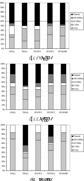
(5) of upper bounds is not selected, and in all experiments, we fixed the timeout of each run to 1000 seconds. As the benchmark set, we adopted three benchmark suites, Random, Uniform, and Locality, a brief description of which could be stated as follows [6]:. 100% 90% 80% Timeout 70%. 100-1000(s). 60%. 10-100(s) 1-10(s). 50%. Random: Each bid Bi is constructed by selecting ki goods from S without replacement and by assigning a bid value vi to it, where ki is a random value drawn from {1, 2, . . . , m′ }, where m′ ≤ m, and vi is a random value drawn from {1, 2, . . . , M ax}.. 0-1(s) 40% 30% 20% 10% 0% LPALL. TRALL. Uniform: Modify Random in such a way that the size of each bid is fixed to a constant k.. STATIC1. STATIC2. DYNAMIC. (a) Random. 100%. Locality: Modify Random in such a way that the goods selected by the bids follow a locality according to the Zipf’s first law [7].. 90% 80% Timeout 70%. 100-1000(s) 10-100(s). 60%. For each suite, we varied the average number of goods in a bid as 3, 6, and 9; the total number of goods as 50, 200, and 350; and the number of bids is 100, 300, 500, and 700; i.e., we prepared 36 instances for each suite. As an initial assessment, we evaluate the performance of the system by assigning LP to all agents (LPALL) or by assigning TRV to all agents (TRVALL). In the experiment, we compare the number of instances (among 36 instances for each suite) for which a given scheme exhibits the better performance than the other scheme. The result is summarized as follows: for LPALL, such number of instances for Random, Uniform, and Locality are 19, 9, and 30, respectively, and for TRVALL, they are 9, 11, and 6, respectively. Thus, we can conclude that LPALL is better than TRVALL for Uniform or Locality, and TRVALL is better than LPALL for Random.. 1-10(s). 50%. 0-1(s) 40% 30% 20% 10% 0% LPALL. TRALL. STATIC1. STATIC2. DYNAMIC. (b) Uniform. 100% 90% 80% Timeout 70%. 100-1000(s) 10-100(s). 60%. 1-10(s). 50%. 0-1(s) 40% 30% 20%. 5.2. Results. 10% 0%. Figure 2 compares the distribution of the computation time for each scheme. We could observe that: • The goodness of two static schemes depends on the class of given instances; e.g., the first scheme is not good for Uniform and Random, and the second scheme is not good for Locality. • The performance of the dynamic scheme is relatively stable independent of the class of instances; e.g., it is as good as LPALL for Uniform and Locality, and it is as good as TRVALL for Random. In order to examine the goodness of the static schemes in more detail, we verified the appropriateness of the policy selected by the schemes. Table 1 shows the number of instances for which an appropriate policy is successfully selected by the schemes, where the selection with probability 0.5 in the second scheme is considered to be successful. As is shown in the table, the first static scheme could not select an appropriate policy except for Locality, which is due to the inaccuracy of estimation at the root of the search tree. Conversely, the goodness of the scheme for Locality is due to the tightness of the estimation at the root, which makes the scheme to always select LP to generate a good solution. In the law, the ith element wi in S is associated with a def P|S| probability pi = 1/(i × Q), where Q = i=1 (1/i). Note that P|S| p = 1 holds by definition. i i=1. LPALL. TRALL. STATIC1. STATIC2. DYNAMIC. (c) Locality. Figure 2: Computation time of each scheme.. On the other hand, the second static scheme could not select an appropriate policy for Locality, although it could make an appropriate selection for Uniform and Random. The badness for Locality is due to the inaccuracy of the number of bids in an optimum solution for the instances contained in Locality. In fact, the actual number of bids contained in an optimum solution is 26,65, 28.54, and 25.83 for Random, Uniform, and Locality, respectively, whereas the estimated number of bids are 30.68, 21.56, and 7.28, respectively. In contrast to the static schemes, the dynamic scheme exhibits a stable performance for all classes of the instances. An advantage of the dynamic scheme is that it allows each agent to have its own policy. In order to examine the impact of this advantage to the performance, we compare the performance of the dynamic scheme with schemes with a fixed percentage of LP policy, where the percentage is varied as 100%, 75%, 50%, 25%, and 0%. Figure 3 illustrates the result for Random (the case of LP with x% is denoted as LP(x) in the figure), and the probability of selecting LP is summarized for each instance in Table 2. Note that this fig-. −11− -5-.
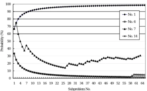
(6) 100. Table 1: The number of instances for which an optimum policy was selected.. Random Uniform Locality. No. 1. 80. static 2 success failed 19 1 27 1 14 22. No. 6. 70 Probability (%). static 1 success failed 10 10 13 15 31 5. 90. No. 7. 60. No. 14. 50 40 30 20 10 0. LP(100). LP(75). LP(50). LP(25). LP(0). Dynamic. 1. 4. 7. 10 13 16 19 22 25 28 31 34 37 40 43 46 49 52 55 58 61 64 Subproblem No.. 1000. Figure 4: Temporal transition of selection probability.. Time (s). 100. 6 10. 1. 0.1 1. 2. 3. 4. 5. 6. 7. 8. 9. 10. 11. 12. 13. 14. 15. 16. Instance No.. Figure 3: Result for dynamic scheme.. ure omits instances that could be solved in one second, and of course, omits instances that could not be solved within 1000 seconds. From the figure, we could observe the superiority of the dynamic scheme. Although there are several instances for which the other schemes outperform the dynamic scheme (e.g., instances No. 6 and 7), we could conclude that the dynamic scheme could select an appropriate policy. To see this in more detail, we evaluated how the probability of selecting LP transits during the execution of the scheme. Figure 4 summarizes the result for bad instances (No. 6 and 7) and good instances (No. 1 and 14). The horizontal axis of the figure represents the sequence number of subproblems sent out to the agents, and the vertical axis represents the probability of selecting LP for the subproblem with a given sequence number. As is shown in the figure, for good instances, it converges to an appropriate policy, although it takes relatively long time before convergence. On the other hand, for bad instances, it often makes a wrong decision, which causes unnecessary vibration of the probability. By a detailed analysis of such instances, we found that such instances could be effectively solved by appropriately solving a specific subproblem, and to efficiently solve them, we have to select a specific policy, whereas the most of the remaining subproblems do not strongly rely on the selection of the policy. An improvement of the dynamic scheme in such a way to incorporate with such a situation is left as a future problem.. Table 2: Probability of selection in Dynamic. Instance No. 1 2 3 4 5 6 7 8 Probability [%] 99 13 93 97 97 4 31 96 Instance No. 9 10 11 12 13 14 15 16 Probability [%] 1 1 39 6 6 1 60 1. Concluding Remarks. In this paper, we proposed a new class of parallel B&B schemes, and described a detail of our first prototype system implemented over eight PC’s. The result of experiments conducted over the prototype system indicates that the dynamic selection of exploring policies could improve the overall performance of the underlying B&B scheme, and it could efficiently support the functional parallelism residing in the original B&B scheme. We are extending the prototype system in such a way that the search space submitted by each node is shared by all nodes participating to the problem solving.. References [1] J. Clausen , M. Perregaard. On the best search strategy in parallel branch-and-bound: Best-First Search versus Lazy Depth-First Search. Annals of Operations Research, 1999, 90(1): 1-17(17), 1999. [2] Y. Fujishima, K. Leyton-Brown, Y. Shoham. Taming the computational complexity of combinatorial auctions: Optimal and approximate approaches. In Proc. IJCAI’99, pages 548–553, 1999. [3] S. Fujita, S. Tagashira, C. Qiao, M. Mito, Distributed Branch-and-Bound Scheme for Solving the Winner Determination Problem in Combinatorial Auctions. In Proc. AINA 2005 , March 28–30, Tamkang University, Taiwan (2005). [4] Portable Parallel Branch-and-Bound Library http://wwwcs.upb.de/fachbereich/AG/ monien/SOFTWARE/PPBB/ppbblib.html [5] Y. Sakurai, M. Yokoo, K. Kamei. An efficient approximate algorithm for winner determination in combinatorial auctions. In ACM Conf. on Electronic Commerce, pages 30–37, 2000. [6] T. Sandholm. Algorithm for optimal winner determination in combinatorial auctions. Artificial Intelligence, 135(1-2): 1–54, 2002. [7] G. K. Zipf. Human Behavior and Principle of Least Effort. Boston: Addison-Wesley (1949).. -−12− 6-E.
(7)
図

関連したドキュメント
2 Combining the lemma 5.4 with the main theorem of [SW1], we immediately obtain the following corollary.. Corollary 5.5 Let l > 3 be
It is suggested by our method that most of the quadratic algebras for all St¨ ackel equivalence classes of 3D second order quantum superintegrable systems on conformally flat
In this paper, under some conditions, we show that the so- lution of a semidiscrete form of a nonlocal parabolic problem quenches in a finite time and estimate its semidiscrete
In this note, we consider a second order multivalued iterative equation, and the result on decreasing solutions is given.. Equation (1) has been studied extensively on the
A monotone iteration scheme for traveling waves based on ordered upper and lower solutions is derived for a class of nonlocal dispersal system with delay.. Such system can be used
Kilbas; Conditions of the existence of a classical solution of a Cauchy type problem for the diffusion equation with the Riemann-Liouville partial derivative, Differential Equations,
By the algorithm in [1] for drawing framed link descriptions of branched covers of Seifert surfaces, a half circle should be drawn in each 1–handle, and then these eight half
The study of the eigenvalue problem when the nonlinear term is placed in the equation, that is when one considers a quasilinear problem of the form −∆ p u = λ|u| p−2 u with
