符号問題のない領域からの量子色力学相図の決定

(1)

九州大学学術情報リポジトリ

Kyushu University Institutional Repository

符号問題のない領域からの量子色力学相図の決定

境, 祐二

九州大学大学院理学府

https://doi.org/10.15017/21708

出版情報：Kyushu University, 2011, 博士（理学）, 課程博士バージョン：

権利関係：

(2)

Determination of the phase diagram of Quantum Chromodynamics

from the regions with no sign problem

Yuji Sakai

Theoritical Nuclear Physics, Department of Physics,

Graduate School of Sciences, Kyushu University

(3)

(4)

Acknowledgements

I would like to express my special gratitude to Prof. Masanobu Yahiro who is teaching and supporting me as a supervisor. By his valu- able suggestions through many discussions, my Master and Doctoral Course become a fruitful and wonderful period in my life. I would like to thank Prof. Masayuki Matsuzaki and Associate Prof. Hiroaki Kouno who gave me a lot of useful comments and helpful discussions on this thesis. Through many discussions, I was able to obtain much beneﬁcial knowledge. I wish to express my deep appreciation to As- sociate Prof. Yoshifumi R. Shimizu, Assistant Prof. Kazuyuki Ogata and Assistant Prof. Takuma Matsumoto. They gave me much important knowledge of Nuclear Physics from all seminars, lessons and discussions. I would like to thank Assistant Prof. Namiko Mitarai for her helpful comments in the Front Researcher Development pro- gram. I would like to thank my friends in the Nuclear Theory Group and other divisions in Kyushu University. This work was supported by the Research Fellowships of the Japan Society for the Promotion of Science (JSPS) for Young Scientists. Finally, I deeply appreciated grateful supports of my families who stood by me and gave me in- telligent advices whenever I was at a loss what to do. Without their supports I never accomplished this great works.

(5)

Abstract

Quantum chromodynamics (QCD) is the theory of the strong interaction between quarks and gluons. The interaction becomes small at high energy, while it does strong at low energy. It is highly expected from the energy dependence that the QCD matter at high temperature T and/or high quark chemical potential µ_q experiences a phase transition from a confined state with the chiral symmetry breaking to a deconfined state with the symmetry restoration. The phase diagram in theT-µ_q plane is relevant to the early universe, compact stars and heavy-ion collisions. The first-principle lattice QCD (LQCD) suffers from the sign problem at finite µq where the integrand of the partition function is complex and LQCD techniques break down. Therefore the QCD phase diagram at finite µ_q is unclear. In this thesis, we propose a new strategy to investigate the QCD phase diagram at finite µ_q. There are some regions with no sign problem, imaginary µ_q and real and imaginary isospin chemical potentials µ_iso. We then propose an analytic continuation from the regions with no sign problem to the real µ_q region with the sign problem by using an effective model that can evaluate the QCD partition function in all the regions. The Polyakov-loop extended Nambu–Jona-Lasinio (PNJL) model is only the effective model that can do this. We show that the PNJL model reproduces LQCD data qualitatively in all the regions, but not quantitatively. We then extend the PNJL model in order to reproduce the LQCD data quantitatively. The QCD phase diagram at realµ_q is predicted by the new model.

(6)

List of Figures

2.1 Schematic picture of the QCD phase diagram . . . 9

3.1 Order parameters in the PNJL model . . . 22

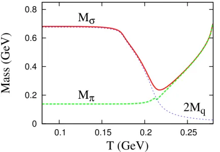
3.3 T dependence of the meson masses . . . 24

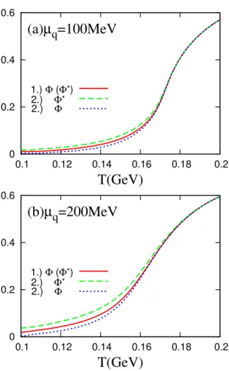
4.1 T dependence of the Polyakov loop and its conjugate . . . 37

4.2 The diﬀerence between the Polyakov loop and its conjugate . . . . 38

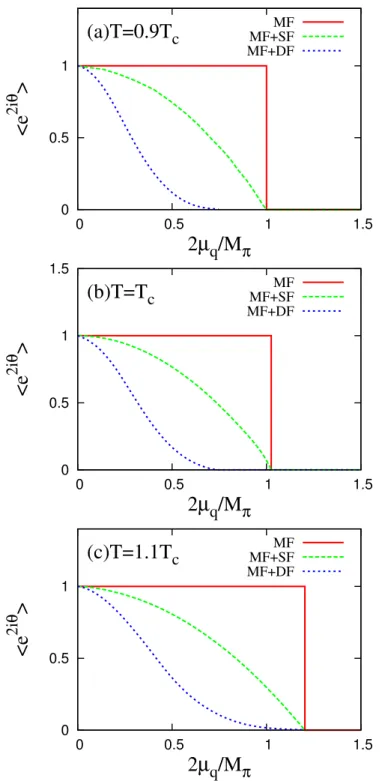
4.3 µ_q dependence of the average phase factor . . . 40

4.4 Comparison of the average phase factor with the LQCD results . . 41

4.5 The average phase factor in the µ_q-T plane . . . 43

4.6 The Polyakov loop dependence of the average phase factor . . . . 43

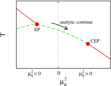
5.1 Schematic picture of the QCD phase diagram in the µ²_q-T plane. . 46

5.2 Predictions for location of the critical endpoint . . . 48

5.3 θ_q dependence of the potential with the ﬁxed phases . . . 51

5.4 θ_q dependence of the thermodynamic potential . . . 56

5.5 θ_q dependence of the Polyakov loop . . . 57

5.6 θ_q dependence of the chiral condensate . . . 58

5.7 θ_q dependence of the quark-number density . . . 59

5.8 θ_q dependence of the meson masses . . . 60

5.9 T dependence of the Polyakov loop at θq=π/3 . . . . 61

5.10 The Polyakov loop in theθ_q-T plane. . . 62

5.11 The phase diagram at imaginaryµ_q . . . 63

(11)

LIST OF FIGURES

5.12 The phase diagram in theµ²_q-T plane . . . 64

5.13 Extrapolation of the chiral phase transition curve . . . 65

5.14 Dependence of CEP on the strength of the vector-type interaction 67 5.15 Impact of the vector-type interaction at imaginary µq . . . 68

6.1 θ_q dependence of the potential . . . 81

6.2 Phase diagram in the θ_iso-θ_q plane at T = 250MeV . . . 82

6.3 θ_I dependence at lower temperature . . . 83

6.4 Thermodynamics in theθ_q-θ_iso plane . . . 85

6.5 LQCD results for the number densities in the θ_q-θ_iso plane . . . . 86

6.6 Comparison of the PNJL model with LQCD . . . 87

6.7 T dependence of number densities . . . 89

6.8 T dependence of |Φ| and σ atθiso=π/2 . . . 90

6.9 Phase diagram in θ_iso-T plane . . . 91

6.10 Pion condensate at real isospin chemical potential . . . 94

6.11 Pion condensate at real isospin chemical potential . . . 94

7.1 Eﬀective vertex in the EPNJL model . . . 100

7.2 T dependence of the order parameters atµ_q= 0 . . . 102

7.3 T dependence of the susceptibilities at µ_q = 0 . . . 102

7.4 T dependence of the order parameters atθ_q =π/3 . . . . 103

7.5 T dependence of the susceptibilities at θq=π/3 . . . . 103

7.6 θq and T dependences of the phase of the Polyakov loop . . . 104

7.7 Phase diagram in θ_q-T plane . . . 106

7.8 Mass dependence of the RW endpoint . . . 107

7.9 Phase diagram in the µ²_q-T plane . . . 108

7.10 T dependence of the order parameters atθ_iso =π/2 . . . . 109

7.11 T dependence of the order parameters at realµ_iso . . . 111

7.12 Phase diagram in theµ_iso-T plane . . . 112

7.13 T dependence of the equation of state . . . 114

(12)

Chapter 1 Introduction

Quantum chromodynamics (QCD) is the theory of the strong interaction between quarks and gluons. The interaction becomes small at high energy, while it does strong at low energy. As a result of the strong interaction, the QCD vacuum has two remarkable phenomena, spontaneous chiral symmetry breaking and confinement. The spontaneous chiral symmetry breaking provides us the mechanism of generation of massive nucleons from light quarks and that of pions as Nambu-Goldstone bosons. The confinement is a phenomenon that color charged particles, quarks and gluons, cannot be isolated. Since the interaction decreases with increasing the energy scale, it is natural to consider that the QCD matter at high energy density undergoes a phase transition from a confined state with the chiral symmetry broken to a deconfined state with the symmetry restored.

The QCD phase diagram in the plane of temperature T and quark chemical potential µ_q provides us many insights of nature. The early universe after the Big Bang would be very hot and thus have experienced the QCD phase transition at high T and low µ_q. The core of compact stellar objects such as neutron stars would be a relevant place for dense QCD matter at low T and high µ_q. Ex- perimentally, the heavy-ion collisions, such as the Relativistic Heavy-ion Collider (RHIC) at BNL, the Large Hadron Collider (LHC) at CERN and Japan Proton Accelerator Research Complex (J-PARC) at JAEA and KEK, provides us with a chance to create hot and/or dense QCD matter. In order to investigate the QCD phase diagram, we have to deal with some nonperturbative methods. Lattice

(13)

i.e., to evaluate the partition function numerically on a spacetime lattice. LQCD provides us many insights at finite T and zero µ_q; for example the chiral phase transition is crossover there. It, however, suffers from the sign problem at finite µq where the integrand of the partition function is complex and thereby LQCD techniques break down. The QCD phase diagram at finiteµ_qis therefore unclear.

In this thesis, we propose a new strategy to investigate the QCD phase diagram at ﬁniteµ_q. There are some regions with no sign problem, imaginaryµ_q, real and imaginary isospin chemical potentials µ_iso. We then propose an analytic continuation from the regions with no sign problem to the real µ_q region by using an eﬀective model that can evaluate the QCD partition function in all the regions.

The Polyakov-loop extended Nambu–Jona-Lasinio (PNJL) model is an eﬀective model that can do this. We show that the PNJL model reproduces LQCD data qualitatively in all the regions with no sign problem, but not quantitatively. We then extend the PNJL model in order to reproduce the LQCD results quantitatively.

This thesis is organized as follows. In Chapter 2, we overview properties of QCD at vacuum and the QCD phase diagram at finite T and µ_q. This shows current states and difficulties in the study of the QCD phase diagram. In Chapter 3, we recapitulate thermal properties of the PNJL model at zero µq. After these introductory chapters, Chapters 4-7 are devoted to our study. In Chapter 4, we investigate the sign problem by using the PNJL model. We evaluate the average phase factor as an indicator of the sign problem. The severe region where the factor is small or zero spreads widely over the phase diagram. It is thus difficult to investigate the phase diagram by LQCD directly. In Chapters 5 and 6, we analyze the imaginary µ_q region and the real and imaginary µ_iso regions with the PNJL model, respectively. For all the regions, the PNJL model reproduces the LQCD data qualitatively, but not for the coincidence between the chiral and deconfinement crossover transitions. In Chapter 7, we extend the PNJL model to solve this problem. The new model reproduces LQCD data quantitatively in all the regions with no sign problem. Finally we predict the QCD phase diagram with the new model.

(14)

Chapter 2 Quantum Chromodynamics

In this chapter we introduce Quantum chromodynamics (QCD) as the fundamental theory of strong interactions. We discuss two important phenomena of QCD vacuum, the spontaneous chiral symmetry breaking and confinement, which play an important role in later parts of this work. We also discuss the QCD phase diagram at finite temperature and finite quark chemical potential [1].

2.1 Quantum Chromodynamics

Quantum Chromodynamics (QCD), the non-Abelian gauge theory with color SU(3)_c gauge invariance, is the theory of the strong interaction. The fundamental degrees of freedom are spin-1 gauge bosons (gluons A_µ), and massive spin-¹₂ fermions (quarks q). Gluons and quarks belong to the adjoint and fundamental representations ofSU(3)_c, respectively. QCD is deﬁned as a ﬁeld theory with the Lagrangian density,

L= ¯q(iγ^µD_µ−m)q− 1

4g²F_µνâ F_a^µν, (2.1) where m is the current quark mass, D_µ =∂_µ+iAâ_µtâ is the covariant derivative with the coupling constant g and tâ is the generators of SU(3)_c satisfying the commutation relations, [tâ, t^b] = ifâbct^c, and the normalization, tr(tât^b) = ¹₂δâb, wherefâbc are the group structure constants. The field strength tensor is defined

(15)

2. Quantum Chromodynamics

the SU(3)_c gauge transformation

q→U(x)q, A_µ→U(x)(A_µ+i∂_µ)U^†(x), (2.2) where U(x) = exp(−iθ^a(x)t^a). Since QCD is renormalizable, its bare parameters g and m depend on the energy scale Q. The renormalization group equation based on the perturbative calculation reads

α(Q²) = g(Q²)

4π = 1

4πβ₀ln(Q²/Λ_QCD), (2.3) where β₀ = _(4π)¹ 2

(11− ²₃N_f)

and N_f is the number of quark flavors. The QCD scale parameter is given by Λ_QCD = κexp(−1/2β₀g²) with the renormalization point κ and determined from experiment to be ΛQCD ≈ 200MeV ≈ 1fm⁻¹. As long as β₀ > 0 (N_f ≤ 16), the running coupling decreases logarithmically at large energy (or short distance) so that the asymptotic freedom of QCD can be realized [2]. In contrast, the coupling increases at low energy and the perturbative calculation breaks down. Quarks have flavors of N_f = 6 with the masses m_u ≈ m_d ≈ 5MeV, m_s ≈ 150MeV, m_c ≈ 1.5GeV, m_b ≈ 5GeV, m_t ≈ 170GeV, respectively. In this thesis, we focus on physics at the energy scale ∼ Λ_QCD and we consider mainly the two-flavor case of u and d, since the influence of heavy quarks is negligible there.

2.2 Symmetries in QCD Lagrangian

Symmetries of Lagrangian are important to describe a main property of theories.

As for QCD, one of important symmetries is the chiral symmetry. In the massless limit m = 0, the QCD Lagrangian density (2.1) is divided into the left- and right-handed quark parts that are the eigenstates of the chirality operator γ₅, q_R/L= ¹₂(1±γ₅)q. In this limit, the QCD Lagrangian is thus invariant under the flavor U(Nf)L×U(Nf)R global transformation, q_R/L → exp (−iθâtâ)q_R/L where tâ is the generator of U(Nf). This is the chiral symmetry. The transformation

(16)

converts the vector and axial-vector ones as

q →e⁻îθâ^V^tâq, q→e⁻îθÂâ^tâ^γ⁵q, (2.4) withθ_V=θ_L =θ_Randθ_A=−θ_L=θ_R. The corresponding conserved currents are vector and axial-vector currents, J_Vâµ = ¯qγ^µtâq and J_Aâµ = ¯qγ^µγ₅tâq, and thereby they have the following relations

∂_µJ_V^aµ = i¯q[m, t^a]q, (a= 0, ..., N_f²−1), (2.5)

∂_µJ_A^aµ = i¯q{m, t^a}γ₅q, (a = 1, ..., N_f²−1), (2.6)

∂_µJ_A^0µ = √ 2/N_f

(

iqmγ¯ ₅q− 2N_f

64π²F_a^µνF˜_µν^a )

, (2.7)

where ˜F_µνâ =ϵµνρσF_a^ρσ(ϵ0123 = 1) is the dual field strength. TheU(1)AcurrentJ_A^0µ is explicitly broken even at m = 0 by the quantum effect that is originated from the non-invariance of the path integral measure under theU(1)_Atransformation.

This gives rise to an unnaturally large η^′ meson mass.

2.3 QCD vacuum structure

Since the QCD running coupling becomes stronger at low energy, quarks and gluons interact nonperturbatively there. There are two remarkable phenomena in the nonperturbative regime, spontaneous chiral symmetry breaking and conﬁnement.

2.3.1 Chiral symmetry breaking

The chiral symmetrySU(Nf)V×SU(Nf)Ain the Lagrangian is broken at vacuum.

Here we consider the N_f = 2 case for simplicity. In nature, there is a triplet of light pseudoscalar mesonsπ, while the parity partner of scalar mesonσhas much heavier mass. This mass gap is explained as spontaneous breaking of the chiral symmetry. For nonperturbative nature, the ground state|0⟩of QCD is symmetric only under the SU(N_f)_V transformation generated by the vector charges Q^a_V =

∫ d³xJ_V^a0, i.e., Q^a_V|0⟩ = 0, but not under the SU(N_f)_A transformation generated

∫ | ⟩ | ⟩ ̸

(17)

energetically degenerate with the ground state|0⟩and which carries the quantum numbers of the corresponding axial charges. These are Nambu-Goldstone bosons of light pseudoscalar mesons. The SU(Nf)A transformation of the pion state, π^a= ¯qiγ5t^aq, is given as, forNf = 2

[Qâ_A,qiγ¯ 5tâq] =−iδâbqq,¯ (2.8) thus the chiral partner of the pseudoscalar mesons is the sigma mesonσ= ¯qq and the expectation value of theσ state is an order parameter of the chiral symmetry,

⟨qq¯ ⟩=⟨q¯_Lq_R+ ¯q_Rq_L⟩. (2.9) The decay amplitude of the pion is written as

⟨0|J_A^aµ(x)π^b(p)⟩

=−ip^µf_πδ^abe⁻^ipx, (2.10) where f_π is the pion decay constant. By combining (2.6) with (2.8), we obtain

⟨0|[

Q¹_A, ∂_µJ_A^1µ]

|0⟩=−i

2(m_u+m_d)⟨qq¯ ⟩, (2.11) where mu and md are u and d quark masses, respectively. The expression on the left-hand side can also be calculated from (2.10) by inserting a complete set of pseudoscalar states in the commutator. Truncating this set by the one-pion states |π^a⟩, one obtains

M_π²f_π² =−m⟨qq¯ ⟩+O(m²), (2.12) where the isospin symmetry is assumed, mu = md = m. The relation (2.12) is called the Gell-Mann–Oakes–Renner relation [7]. Here inserting f_π ≈ 93MeV, M_π ≈ 140MeV and m ≈ 5MeV into (2.12), we obtain ⟨qq¯ ⟩ ≈ −(250MeV)³ and the chiral symmetry is spontaneously broken at vacuum.

(18)

2.3.2 Conﬁnement

Another important aspect of nonperturbative QCD is quark conﬁnement. The mechanism is however much less known. Conﬁnement is the phenomenon that all color charges are completely screened in the far away region of the color source.

In the heavy quark limit, confinement means that a system with a static color source and a static color sink at infinite separation has an infinite free energy.

More precisely, the free energy FQQ¯ of a heavy quark ¯QQ pair is proportional to the separation R of the two quarks. The free energy is obtained from the expectation value of the Wilson loop [8]

W(C) = Tr [

Pexp (

−i I

C

A_µdx^µ )]

, (2.13)

where the integral is made over a closed pathC andPdenotes the path ordering.

In order to relate the Wilson loop to the free energy, we consider the process where a heavy static ¯QQ pair is created at x₀ = 0, propagates to time x₀ = T → ∞, and then is annihilated. The Euclidian amplitude for the process is obtained as

⟨QQ¯ e⁻^HTQQ¯⟩

=

∫

DAâ_µe⁻^S⁻ⁱ^∫Ââ^µ^Jâµ^d⁴^x =e⁻^F^QQ^¯ ^(R)T, (2.14) whereHis the Hamiltonian andFQQ¯ is the free energy. The currentJâµ describes the closed path C of the creation and annihilation of the QQ¯ pair. We take the current Jâµ = H

Cdz^µt^aδ⁴(x−z) corresponding to a quark Q moving along the path C,

e⁻^F^QQ^¯ ^(R)T =

∫

DAâ_µe⁻^S⁻ⁱ^H^CÂâ^µ^tâ^dx^µ =⟨W(C)⟩. (2.15) Evaluating the expectation value of the Wilson loop, we thus get the free energy of a heavy static particle-antiparticle pair. The free energy proportional to the distance does not allow the flux to spread over infinite space. The factor of the proportionality is called string tension.

(19)

2.3.3 Relation between two phenomena

The chiral symmetry is realized only in the limit of light quark. Meanwhile, the confinement is well defined only at heavy quark masses. Thus the two phenomena can be considered in the opposite limits. Here we comment on the simple argument about the relation between the two phenomena. An argument [4] made by Casher is that the chiral symmetry should be broken in the confinement phase.

The argument is simple and transparent. Suppose quarks are confined in hadrons and the attraction is chiral invariant. In a semi-classical description a bound state is constructed by superposing paths where the bound quarks have to reverse its direction of motion. Since the chirality, that is helicity in massless limit, is conserved in the interaction, the force can flip neither the spin nor the direction of motion due to the helicity conservation. In compensation for the chirality the chiral condensate has a non-zero expectation value and then the chiral symmetry is spontaneously broken in the confinement phase. Another argument [5] is based on the anomaly matching condition proposed by ’t Hooft [6]. Some of the elec- troweak anomalies are canceled between quarks and leptons. Since the leptonic anomaly is unchanged in the confinement phase, the hadrons must represent the flavor anomalies of QCD and ensure the cancellation of the leptonic anomaly. We consider flavor currents such as a left-handed current J_µ = ¯qξ(1−γ₅)γ_µq where ξ is some combination of the generators of SU(N_f) with tr(ξ³)̸= 0. This current has an anomaly expressed as

r^αΓ_µνα(p, q, r) = i g²

4π²tr(ξ³)ϵ_µνβγp^βq^γ, (2.16) Γ_µνα(p, q, r) =

∫

d⁴x₁d⁴x₂e^ipx¹^+iqx²⟨J_µ(x₁)J_ν(x₂)J_α(0)⟩ (2.17) where (p+q+r)^α = 0. This amplitude Γ_µνα has massless poles likep², q² orr². Thus the current J_µ has to create massless states, that is, the Nambu-Goldstone boson due to the spontaneous chiral symmetry breaking.

(20)

2.4 QCD phase diagram

Since the QCD running coupling decreases with respect to increasing the energy scale, it is natural to consider that the QCD matter at high energy density undergoes the phase transition from a conﬁned state with the chiral symmetry breaking to a deconﬁned state with the chiral symmetry restoration. The former (latter) is called the hadron (quark-gluon plasma: QGP) phase. Since the intrinsic scale of QCD is Λ_QCD ∼ 200MeV, the QCD phase transition may take place around temperature T ∼ Λ_QCD or the baryon number density ρ^1/3_B ∼ Λ_QCD = 1fm⁻¹. In the early universe about 10⁻⁵s after the Big Bang, the universe would have

QCD

Quark-Gluon Plasma Temperature

Color Superconductor Quark Chemical Potential Hadron Phase

Figure 2.1: Schematic picture of the QCD phase diagram.

experienced the QCD phase transition. The core of compact stellar objects such as neutron stars thus would be the relevant place where dense QCD matter at low temperature is realized. For asymptotically high density, the QCD ground state forms a condensate of quark Cooper pairs, namely the color superconductor.

Since quarks have color and ﬂavor quantum numbers, the color superconductor phase has a rich structure. Experimentally, the heavy-ion collisions such as the Relativistic Heavy-ion Collider (RHIC) at BNL, the Large Hadron Collider (LHC)

(21)

and KEK provides us with a chance to create hot and/or dense QCD matter [3].

Figure 2.1 sketches a schematic picture of the QCD phase diagram in the plane of temperature T and quark chemical potential µq. At present, our knowledge is limited only in asymptotically high µq region, where the perturbative calculation is available, and small µ_q/T ≪1 region, where the numerical calculation on lattice is available as explained in Sec. 2.6.

2.5 Thermodynamics of QCD

For QCD in equilibrium with volume V, temperature T and quark chemical potential µq, the partition function of the grand-canonical ensemble Z(T, µq) is deﬁned as

Z(T, µ_q) = tr (

e⁻^{β( ˆ}^H⁻^µ^q^N^ˆ^q⁾ )

, (2.18)

whereβ = 1/T and ˆH and ˆN_q are the Hamiltonian and the quark-number operators, respectively. The thermodynamic potential is deﬁned as Ω =−_V^T lnZ. The partition function (2.18) is expressed as a Euclidian functional integral

Z(T, µ_q) =

∫

Dq¯DqDA_νexp [

−

∫ _β

0

dτ

∫

d³x(LE−µ_qqγ¯ ₄q) ]

, (2.19) whereLEdenotes the Lagrangian density in the Euclidian spacetime. Quarks and gluons satisfy antiperiodic and periodic boundary conditions in τ, respectively.

Since the τ direction is compacted, the momentum integral is replaced as

∫ d⁴p (2π)⁴

T̸=0

−−→ 1 β

∑

n

∫ d³p

(2π)³ (2.20)

with the momentump= (p, ω_n) whereω_n= 2nπT for gluons andω_n= (2n+1)πT for quarks. From now on we work in Euclidean spacetime without exception. The Wilson loop (2.13) with the path connecting two points at τ = 0 and β is then rewritten into

⟨W⟩=⟨tr_cL^†(R)tr_cL(0)⟩=e⁻^F^QQ^¯ ^(R)β, (2.21)

(22)

whereFQQ¯ (R) is the free energy of heavy quarks with the separationR. Here the contributions from two paths in the opposite space direction at τ = 0 and β are canceled out each other, note that the τ direction is compacted. The Polyakov loop Φ [9] is deﬁned by

Φ(x) = 1

3tr_cL(x), L(x) =Pexp (

−i

∫ β 0

A₄(τ,x)dτ )

, (2.22)

where P denotes the path ordering. Therefore the Polyakov loop Φ(x) is related to the free energyFQQ¯ at temperatureT of two static color sources ¯QandQwith a spatial separation R [10]. In the limit |R| → ∞, the free energy is reduced to

FQQ^∞¯ =−Tln|⟨Φ⟩|². (2.23) This expression can be related to the free energy of a single quark, F_Q^∞, and a single antiquark, F_Q^∞_¯ . Consequently, ⟨Φ⟩is an order parameter for the conﬁnement.

In the confinement phase, the free energy is infinite so that⟨Φ⟩= 0, while⟨Φ⟩ ̸= 0 in the deconfinement phase. The Polyakov loop is also an order parameter of the Z3 symmetry [11] that is the center elements of color SU(3)c, zk = e⁻^2πik/3 for integer k. Under a non-periodic gauge transformation U_k(x) = [z_k]^{τ /β}, the temporal gauge field is shifted asA₄ →A₄+^2πk_3β so that the Polyakov loop is changed as Φ → z_kΦ. The gauge fields satisfy the periodic boundary condition and the Z3 symmetry is exact in pure gauge limit. The boundary condition for quarks is however changed as q(β,x) = z_kq(0,x) under the transformation so that the Z3

symmetry is explicitly broken in the presence of quarks.

2.6 Lattice QCD

In order to investigate the QCD phase diagram, we have to deal with some nonperturbative methods. Only a reliable method to do this is lattice QCD (LQCD) where the partition function (2.19) is evaluated numerically on the spacetime lattice with a lattice spacingaby using importance sampling techniques. In LQCD, the ingredients are the link variablesU_µ(n) = e⁻^iaA^µ⁽ⁿ⁾ that connect the neighbor

(23)

analytically:

Z =∑

n

∑

µ

detD[U]e⁻^S^g^[U], (2.24)

where D[U] tends to the Dirac operator γ_νD_ν + m − µ_qγ₄ in the continuum limit. For a lattice with N_s (N_t) sites in each spatial (temporal) direction, the total number of integration is N_s³ ×N_t×N_U where N_U = 4 ×8 is degrees of freedom of the link variables at a point. For such a high-dimensional integral, Monte-Carlo methods with importance sampling are suitable where the sampling is generated with a probability proportional to detD[U]e⁻^S^g^[U]. For ﬁnite quark chemical potential µ_q, the probability is no longer positive due to the property of the Dirac operator

[detD(µ_q)]^∗ = det (γ_νD_ν +m−µ_qγ₄)^†

= det[ γ₅(

γ_νD_ν +m+µ^∗_qγ₄) γ₅]

= detD(−µ^∗_q), (2.25) so that the importance sampling techniques break down for ﬁnite µ_q. This is called the sign problem. Several approaches have been proposed so far to circumvent the diﬃculty; for example, the Taylor-expansion method [13], the reweighting method [12], and the analytic continuation from imaginaryµ_qto real µ_q [34; 35; 36; 37]. The Taylor-expansion method has the convergence problem, i.e., the radius of convergence is limited toµ_q/T <1. In the reweighting method, an expectation value of operator O at µ_q ̸= 0 can be rewritten in terms of an ensemble average at µ_q= 0:

⟨O⟩µq =⟨OR(µ_q)⟩0

/⟨R(µ_q)⟩0, (2.26)

whereR(µ_q) = detD(µ_q)/detD(0) is called the reweighting factor. The reweighting method has the overlap problem that the factor R is small in addition to the sign problem. For imaginary µ_q, there is no sign problem because of the relation (2.25). Quantities evaluated in LQCD at imaginaryµ_qcan be continued to realµ_q by some analytic functions. The truncation of the functions, however, limits the range of applicability of this method. All the methods are still far from perfection

(24)

and the QCD phase diagram at ﬁnite µ_q is still under discussion.

(25)

Chapter 3 Polyakov-loop extended

Nambu–Jona-Lasinio model

In the previous chapter, we discussed the QCD phase diagram. The first-principle lattice QCD (LQCD) is only a reliable method to investigate such a nonperturbative region, however it has the sign problem at finite quark chemical potential. As an approach complementary to LQCD, many effective models have been proposed so far. In the QCD phase diagram, important phenomena are chiral symmetry restoration and deconfinement. Recently an effective model which can treat both the phenomena was proposed. The model is call the Polyakov-loop extended Nambu–Jona-Lasinio (PNJL) model. In this chapter, we review properties of the PNJL model at finite temperature and zero chemical potential.

3.1 PNJL Model

The Nambu–Jona-Lasinio (NJL) model [14] has a long history and has been used extensively to describe the dynamics and the thermodynamics of light hadrons, including investigations of the phase diagrams [15]. Such a schematic model oﬀers a simple and practical illustration of the mechanism of the spontaneous chiral symmetry breaking that is a key feature of low-energy QCD. The NJL model is based on an eﬀective Lagrangian of quarks that interact through local current- current couplings, assuming that gluonic degrees of freedom can be frozen into

(26)

3. PNJL model

pointlike effective interactions between quarks. The gluonic correlation length calculated in lattice QCD (LQCD) [16] is small, say ∼ 0.2 fm, compared with a characteristic momentum scale Λ⁻_QCD¹ ≈1 fm. Consider the non-local interaction between two quark color currents, Jâµ = ¯qγ^µtâq, where tâ are the generators of the color SU(3)_c gauge group. The contribution of this current-current coupling to the action is

S_int =−1 2

∫

d⁴xd⁴yJâµ(x)Dâb_µν(x−y)J^bν(y), (3.1) whereDâb_µν is the full gluon propagator. ThisS_int generates the familiar one-gluon exchange between quarks and maintains its higher interactions. Since the gluonic correlation length is much shorter than the typical momentum scale of quarks, the interaction can be approximated by a local coupling between their color currents

S_int =−G_c

∫

d⁴xJâµ(x)J_µâ(x). (3.2) By integrating out gluon degrees of freedom and absorbing them in the four- quark interaction S_int, the local SU(3)_c gauge symmetry is now reduced to a global one in the NJL model. The interaction action S_int evidently preserves the chiral symmetry in the massless limit. A Fiertz transformation of the color current-current interaction (3.2) produces a set of exchange terms acting in quark- antiquark channels: for the two-flavor case,

S_int → −G_s

∫

d⁴x[(¯qq)²+ (¯qiγ₅⃗τ q)²] +· · · , (3.3) where ⃗τ are the isospin SU(2) Pauli matrix. The color-singlet pair of scalar- isoscalar and pseudoscalar-isovector operators (3.3) is a minimal subset satisfying the chiral symmetry. The four-quark interaction (3.3) is the starting point of the NJL model. The NJL model illustrates the spontaneous chiral symmetry breaking, that is, the generation of massive quasiparticles from light quarks and that of pions as Nambu-Goldstone bosons. Despite of the success to describe the chiral symmetry breaking, the NJL model lacks the conﬁnement mechanism, a key feature of low-energy QCD besides the chiral symmetry breaking. The

(27)

3. PNJL model

deconﬁnement phase transition is characterized by spontaneous breaking of the Z3 center symmetry of colorSU(3)_cas discussed in Sec. 2.5. The order parameter is the Polyakov loop

Φ(x) = 1

3tr_cL(x), L(x) = Pexp (

−i

∫ β 0

dτ A₄(x, τ) )

, (3.4)

whereA₄ is the temporal gauge field andPdenotes path ordering. The Polyakov- loop extended NJL (PNJL) model, recently proposed in Ref. [64], can describe the spontaneous breaking of the chiral symmetry and the deconfinement mechanism simultaneously. In the PNJL model, the coupling of the Polyakov loop Φ to the quark fields q is accomplished by the minimal gauge coupling procedure, where the temporal component of the gauge field is assumed to be spatially constant and the other components are neglected. Its basic ingredients are the NJL type four-quark contact interaction and the coupling to a spatially-constant temporal gauge field representing the Polyakov loop. The model Lagrangian is obtained in the Euclidian spacetime as

L= ¯q(γ_νD_ν+m₀)q−G_s[(¯qq)²+ (¯qiγ₅⃗τ q)²] +U_Φ, (3.5) where Dν = ∂ν +iA4δ4ν and m0 is the current quark mass. UΦ is an eﬀective potential for the Polyakov loop and is called as the Polyakov potential. In the PNJL model, the chiral and deconﬁnement transitions are described as the four- quark interaction and the Polyakov potential, respectively.

3.2 Polyakov potential

In the PNJL model the gluonic dynamics is incorporated into the Polyakov potential UΦ. The functional form is inspired by the strong coupling expansion [17].

In the strong coupling limit, the eﬀective action in terms of the Polyakov loop reads

S_L =−e⁻^σaβ∑

n.n.

tr_cL^†(x_i)tr_cL(x_j), (3.6)

(28)

3. PNJL model

which describes a hopping interaction between adjacent Polyakov loops. Here a and σ are the lattice spacing and the string tension, respectively. This action is similar to the nearest neighbor interaction of a spin system of the Polyakov loop.

The partition function of the action is Z_Φ =

∫

DL e⁻^S^L =e⁻^V^Φêff, (3.7) where DL represents the functional integral with the group invariant (Haar) measure, i.e., the Faddeev-Popov determinant. In the mean field approximation, the effective potential (per volume) for the Polyakov loop is obtained as

V_Φ^eﬀ =−54e⁻^σaβΦ^∗Φ−lnMHaar, (3.8) where the Haar measure for the SU(3)_c group is given by

MHaar = 1−6Φ^∗Φ + 4(Φ^∗³+ Φ³)−3(Φ^∗Φ)² (3.9) in the Polyakov gauge where the temporal gauge field is diagonal and static. The second term in (3.8) favors the confined state at Φ = 0, while the first term does the deconfined state Φ = 1. Thus, the Haar measure could play an essential role in the realization of the confinement [18]. Together with the two terms, a phase transition takes place. Here, we distinguish the conjugate of the Polyakov loop, Φ^∗ = ⟨¹₃trcL^†⟩, from Φ; they are just identical at zero quark chemical potential, µ_q= 0, but a difference between them arises at finiteµ_q. The difference has much to do with the sign problem as discussed in Sec. 4.6.1. Inspired by the functional form from the strong-coupling analysis, we adopt the following ansatz to fit the pressure in the pure gluonic sector [25]:

U_Φ =−a(T)

2 Φ^∗Φ +b(T) ln[1−6Φ^∗Φ + 4(Φ^∗³+ Φ³)−3(Φ^∗Φ)²]. (3.10) The parameters are determined to reproduce the LQCD data [19] in the pure gauge limit, a(T)/T⁴ = 3.51−2.47t+ 15.2t² and b(T)/T⁴ = −1.75t³ with t = T₀/T. The ﬁrst term in a(T) is constrained by the Stefan-Boltzmann limit at

(29)

3. PNJL model

LQCD yields T₀ = 270 MeV in pure gauge limit.

3.3 Thermodynamics in the PNJL model

3.3.1 Thermodynamic potential

Given the PNJL model Lagrangian (3.5), we can discuss the thermodynamics.

We start with the partition function Z =

∫

dA₄Dq¯Dq exp [

−

∫

d⁴x(L−µ_qqγ¯ ₄q) ]

, (3.11)

where the temporal gauge field A4 is assumed to be spatially and temporally constant in the PNJL model. For proceeding the path integral of the quark field q, we introduce the auxiliary bosonic fields, σ and ⃗π.

N=

∫

DσDπ_iexp(

−G_s[(¯qq−σ)²+ (¯qiγ₅τ_iq−π_i)²])

. (3.12)

Inserting the constant terms in the partition function, we can convert the four- quark interaction to the bosonic one. The path integration over the quark ﬁelds can be carried out and then the partition function is obtained as

Z =

∫

dA₄DσDπ_i e⁻^S^bos, (3.13) with the bosonized action

S_bos=−ln det[β(γ_νD_ν +M_q−µ_qγ₄)] +

∫ d⁴x(

G_s[σ²+⃗π²] +U_Φ)

, (3.14) where the symbol det denotes the functional determinant andMq=m0−2Gs(σ+ iγ₅τ_iπ_i) is the dynamical quark mass. We evaluate the partition function (3.13) in the mean field approximation. In the mean field approximation, the field variables φ are replaced by the mean fields ¯φ. The mean field configurations are spatially and temporally constants that contribute mostly to the path integral.

In this approximation, the partition function is reduced to Z =e⁻^{S( ¯}^φ) =e⁻^βV^Ω, where Ω is the thermodynamic potential and V is the volume. The mean ﬁelds

(30)

3. PNJL model

are determined by minimizing the potential, i.e., the stationary condition

∂Ω

∂φ = 0 for φ = ¯φ. (3.15)

For finite quark chemical potential µq, the action (3.14) is in general complex. It is then difficult to take the configurations that most contribute to the partition function, i.e., the sign problem. We address this problem in Chapter 4. Here we consider only the zeroµ_qcase where the action remains real. The thermodynamic potential Ω in the mean field approximation is obtained as

Ω_mf =−2N_f1 β

∑

n

∫ _Λ d³p

(2π)³tr_cln[

(ω^c_n)²+p²+M_q²]

+G_s[σ²+π²_i] +U_Φ, (3.16) where ω_n^c =ω_n−iµ_q−A₄ and ω_n = (2n+ 1)πT are the Matsubara frequencies for quarks. Here we introduce the momentum cutoff Λ since the PNJL model is nonrenormalizable. We assume that there is no pion condensate ⟨π_i⟩ = 0, which is justified whenever the isospin chemical potential is zero. By using some technique for the sum, the first term of the potential becomes

ln[

(ω_n^c)² +p²+M_q²]

=[

Eq+ ln(

1 +Le⁻^β(E^q⁻^µ^q⁾) + ln(

1 +L^†e⁻^β(E^q^+µ^q⁾)]

(3.17) with the quasiparticle energy E_q = √

p²+M_q² and L = e⁻^iβA⁴ in the Polyakov gauge. Furthermore the color trace is explicitly taken to be a form of

tr_cln(

1 +Le^−β(E^q^−µ^q⁾)

= ln(

1 + 3Φe^−β(E^q^−µ^q⁾+ 3Φ^∗e^−2β(E^q^−µ^q⁾+e^−3β(E^q^−µ^q⁾)

, (3.18) tr_cln(

1 +L^†e⁻^β(E^q^+µ^q⁾)

= ln(

1 + 3Φ^∗e⁻^β(E^q^+µ^q⁾+ 3Φe⁻^2β(E^q^+µ^q⁾+e⁻^3β(E^q^+µ^q⁾)

. (3.19) From the stationary condition for σ, we can get the relation

⟨σ⟩=−4N_f1 β

∑

n

∫ d³p (2π)³tr_c

( M_q

(ω_n^c)²+p² +M_q² )

=⟨qq¯ ⟩, (3.20) that is the self-consistence condition in the PNJL model. This relation connects the scalar meson ﬁeld σ to the chiral condensate.

(31)

3. PNJL model

3.3.2 Meson properties

Here we consider the mesonic fluctuations around the mean fields. We write σ(x) = ⟨σ⟩+δσ(x), π_i(x) = δπ_i(x) and expand the bosonized action (3.14) per volume around the mean field up to the second order of the mesonic fluctuations δσ, δπ

S_bos=S_bos⁽⁰⁾ +S_bos⁽²⁾, (3.21) whereS_bos⁽⁰⁾ corresponds to the mean ﬁeld part (3.16). The second term is obtained as

S_bos⁽²⁾ = 1 2

∫ d⁴p (2π)⁴

(F⁺(p²)δσ(p)δσ(−p) +F⁻(p²)δπ_i(p)δπ_i(−p))

, (3.22) where p = (p, ω_m) with the Matsubara frequencies ω_m = 2mπT for meson. The inverse meson propagators, F⁺(p²) = _V¹δσ(p)δσ(−p)^δ²^S^bos and F⁻(p²) = _V¹ δπ(p)δπ(−p)^δ²^S^bos , are obtained as

F^±(p²) =

∫ d⁴q (2π)⁴tr[

Γ^±S(q⁺)Γ^±S(q⁻)]

+ 2G_s= (2G_s)² (

N^±I(p²) + m₀ 2GsMq

)

, (3.23) where S(q^±) = (iγ ·q^±+M_q)⁻¹ is the quark propagator with q^± =q±p/2 and

q = (q, ω_n^c). The trace is taken over Dirac, ﬂavor and color. The symbol +(−) represents the σ (π_i) meson mode and N⁺ = p² −4M_q², N⁻ = p², Γ⁺ = 1, Γ⁻ =iγ₅τ_i and

I(p²) = 2N_f

∫ d⁴q

(2π)⁴tr_c 1

[(q⁺)²+M_q²][(q⁻)²+M_q²]. (3.24) The pion mass M_π is determined by the pole of the pion propagator, while the quark-pion coupling constant g²_π¯_qq is by the residue of the pion pole,

M_π² =g_π²_qq_¯ m₀

2G_sM_q, g_π⁻_qq_¯² =I(p²). (3.25) This relation shows that when the chiral symmetry is broken in the massless limit m₀ = 0, the pion behaves as the massless Nambu-Goldstone boson. The