Kazuto Fukuchi 1 , Jun Sakuma 1 , and Toshihiro Kamishima 2
1
University of Tsukuba, 1-1-1 Tennodai, Tsukuba, Ibaraki, 305-8577 Japan [email protected] , [email protected]
2
National Institute of Advanced Industrial Science and Technology (AIST), AIST Tsukuba Central 2, Umezono 1-1-1, Tsukuba, Ibaraki, 305-8568 Japan
[email protected]
Abstract. With recent developments in machine learning technology, the resulting predictions can now have a significant impact on the lives and activities of individuals. In some cases, predictions made by machine learning can result unexpectedly in unfair treatments to in- dividuals. For example, if the results are highly dependent on personal attributes, such as gender or ethnicity, hiring decisions might be deemed discriminatory. This paper investigates the neutralization of a probabilis- tic model with respect to another probabilistic model, referred to as a viewpoint. We present a novel definition of neutrality for probabilistic models, η-neutrality, and introduce a systematic method that uses the maximum likelihood estimation to enforce the neutrality of a prediction model. Our method can be applied to various machine learning algo- rithms, as demonstrated by η-neutral logistic regression and η-neutral linear regression.
Keywords: neutrality, fairness, discrimination, logistic regression, linear regression, classification, regression, social responsibility.
1 Introduction
With recent developments in machine learning technology, the resulting predic- tions can now have a significant impact on the lives and activities of individuals.
In some cases, there are safeguards in place so that the predictions do not cause unfair treatment, discrimination, or biased views of individuals [1]. The following two examples describe situations in which predictions made by machine learning can cause unfair treatments.
Example 1 (hiring decision). A company collects personal information from employees and job applicants; this information includes age, gender, race or ethnicity, place of residence, and work experience. The company uses machine learning to predict the work performance of the applicants, using information collected from employees. The hiring decision is then based on this prediction.
Example 2 (personalized advertisement and recommendation). A com- pany that provides web services records user behavior, including usage history
H. Blockeel et al. (Eds.): ECML PKDD 2013, Part II, LNAI 8189, pp. 499–514, 2013.
c Springer-Verlag Berlin Heidelberg 2013
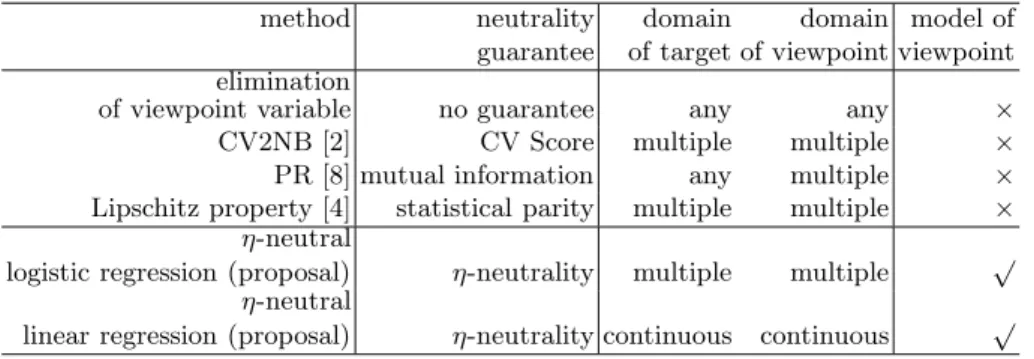
Table 1. Summary of learning algorithms with neutrality guarantee method neutrality domain domain model of
guarantee of target of viewpoint viewpoint elimination
of viewpoint variable no guarantee any any ×
CV2NB [2] CV Score multiple multiple ×
PR [8] mutual information any multiple × Lipschitz property [4] statistical parity multiple multiple ×
η-neutral
logistic regression (proposal) η-neutrality multiple multiple √ η-neutral
linear regression (proposal) η-neutrality continuous continuous √
and search logs, and uses machine learning to predict user attributes and prefer- ences. The advertisements or recommendations displayed on web pages are thus personalized so that they match the predicted user attributes and preferences.
In the hiring-decision example, if the results are highly dependent on per- sonal attributes, such as gender or ethnicity, hiring decisions might be deemed discriminatory. In the second example, when recommendations are accurately pinpointed to sensitive issues, such as political or religious affiliation, the result may be increasingly biased views. This is known as the problem of the filter bubble [10]. For example, suppose supporters of the Democratic Party wish to read news articles related to politics. If the recommended articles are all related to their party and are absent of criticism, they may develop a biased view of the political situation. In the web-service example, showing advertisements that suit the user’s attributes, such as gender or age, would improve the service for some users. Other users, however, may object to advertisements that are apparently based on their race, ethnicity, or gender. Thus, it is difficult to clearly distinguish personalization from discrimination.
We now introduce some terms that will be useful in the following discussion.
The input and output of a prediction model are referred to as input variables (e.g., race, ethnicity, or web-usage history) and target variables (hiring decisions or website recommendations). Factors that might result in discrimination or bias are referred to as viewpoint variables (e.g., race, ethnicity, or political affiliation).
The objective of machine learning is to learn prediction functions that predict target variables from given examples. In the example above, if the viewpoint variables (e.g., race or ethnicity) are dependent on the predicted target variables (e.g., hiring decisions), the prediction function cause unfair treatment. In this paper, we introduce a systematic way to remove this dependency from prediction models and neutralize them with respect to a given viewpoint.
1.1 Related Works
Several techniques that take account of fairness or discrimination have recently
received attention [4][6][12]. One of the easiest ways to suppress unfair treatment
is to remove the values of the viewpoint from the input values before the learning process with the prediction model. If there is no correlation between the input and viewpoint variables, no discrimination or bias will appear after elimination.
However, if another input variable is dependent on the viewpoint variable, then even after the viewpoint values are eliminated, the target variable will retain dependency on the viewpoint variable (Table 1, line 1). For example, assume that the race or ethnicity attribute is eliminated in Example 1. Even so, hiring decisions may be dependent on race or ethnicity if there is a correlation between individuals’ addresses and their race or ethnicity; this is known as the redlining effect [2][11].
Calders et al. presented the Calders–Verwer 2 Naive Bayes method (CV2NB), which proactively removes the redlining effect [2]. Let y ∈ { y + , y − } be the binary target variable, and let v ∈ { v + , v − } be the binary viewpoint variable. Then, the Calders–Verwer (CV) score is defined by CV( D ) = p(y + | v + ) − p(y + | v − ). The CV2NB modifies the naive Bayes classifier in such a way that the CV score becomes zero with respect to the given examples D . The CV2NB guarantees the elimination of discrimination in terms of the CV score. The limitation of the CV2NB is that it cannot be used when the target or viewpoint variables are continuous. Related to the CV2NB, it has been shown [14] that positive CV scores do not necessarily cause discrimination in some situations. There is also a method [9] that uses the kth-nearest neighbor to test for the existence of discrimination. Both these methods are based on the CV2NB, so they share its limitations.
Kamishima et al. have introduced the prejudice remover regularizer (PR) for fairness-aware classification [8]. The PR regularizer penalizes the loss function if there is a high correlation between the target variable and the viewpoint variable.
The penalty is evaluated based on the information that is shared by the target variable y and the viewpoint variable v. This penalty function can work with a continuous target variable if it is approximated by a histogram, as demonstrated by Kamishima et al. [7]. Continuous viewpoint variables, however, cannot be treated by the PR method.
Dwork et al. have presented a classification method that uses a fairness-aware framework, in which statistical parity is used as the measure of fairness [4]. Intu- itively, statistical parity occurs when the demographics of those receiving positive (or negative) classifications are identical to the demographics of the population as a whole. In their fairness-aware framework, the classification is made to be fair by minimizing the empirical risk while satisfying certain constraints that are called the Lipschitz property. As is the case with the CV2NB and PR meth- ods, this framework assumes that the viewpoint variables are binary or multiple;
continuous viewpoint variables are not considered.
1.2 Our Contribution
Modeling Viewpoint Variables. In this manuscript, we provide a method to
neutralize the target prediction model with respect to a probabilistic model of
a given viewpoint. Existing methods assume the viewpoint is observed and is
explicitly provided in the input, but this is not always the case. For instance, consider the recommendation of articles neutralized with respect to political affiliation, as in Example 2. Political affiliation is not explicitly included in the input, but given as input the logs of keyword searches or subscribed news articles, modern machine learning techniques can easily predict party affiliation. In such a case, our method neutralizes the target prediction model with respect to the probability model of such a “hidden viewpoint”.
In order to neutralize a model with respect to a viewpoint, we represent the viewpoint as a probabilistic model and define η-neutrality (Section 2), which is a measure of the dependency of the target prediction model on the viewpoint prediction model. With η-neutrality, we can check the neutrality of a target prediction model with respect to any hidden viewpoint, as long as we have a probabilistic model of the viewpoint variable (Table 1, the rightmost column).
Furthermore, since η-neutrality is measured with respect to probabilistic mod- els, the neutrality of the prediction model with respect to unseen examples is expected to be effectively guaranteed, and this is demonstrated by experiments (Section 5).
Maximum Likelihood Estimation with η-Neutrality. Following the defini- tion of η-neutrality, we introduce a systematic method that removes this depen- dency from the prediction model obtained by the maximum likelihood estimation (Section 2). Our methods can treat target and viewpoint variables that are ei- ther discrete (Table 1, line 5) or continuous (Table 1, line 6), as demonstrated by η-neutrality with logistic regression (Section 3) and linear regression (Section 4).
The effectiveness of our methods is examined by both artificial and real datasets in Section 5.
2 η -Neutrality
We propose a novel definition of neutrality, η-neutrality. We then present a gen- eral maximum likelihood estimation method that has a guarantee of neutrality.
Let D = { (x i , y i ) ∈ X × Y} N i =1 be a set of training examples that are assumed to be i.i.d. samples drawn from a probability distribution Pr(X, Y ). The random variables X and Y are referred to as the input and target, respectively. In the following discussion, the prediction function of the target variable is represented as a probabilistic model f (Y | X ; θ) = Pr(Y | X ), parametrized by θ. The target prediction model can be obtained by minimization of the negative log-likelihood with respect to the parameter θ:
θ ∗ = argmin θ∈Θ L(θ), where
L(θ) = −
( x
i,y
i) ∈D
ln f (y i | x i ; θ). (1)
2.1 Definition of η -Neutrality
In addition to the input random variable X and the target random variable Y , we now introduce the viewpoint random variable V . Let V be the domain of V . The realized values of the variables are denoted by the corresponding lowercase letters. Thus, the random variable X can take the value x. In the following discussion, we assume the input random variable X is continuous. We can treat a discrete X by replacing the integral with a sum. For Y and V , the discussion below is valid for both discrete and continuous variables.
As we did for the target random variable, we assume that the prediction model of the viewpoint variable is represented as a conditional probability Pr(V | X).
Noting that the values of the target and the viewpoint variables are predicted independently, the joint probability is
Pr(X, Y, V ) = Pr(X )Pr(Y | X)Pr(V | X ).
With this assumption, we consider the dependency of the target random vari- able Y and the viewpoint random variable V . When V and Y are statisti- cally independent, for any y ∈ Y and v ∈ V , Pr(v, y)/Pr(v)Pr(y) = 1. When Pr(v, y)/Pr(v)Pr(y) > 1, v and y are more dependent than independent. Hence, our neutrality definition is defined as the ratio of the marginal probabilities, as follows.
Definition 1 (η-neutrality). Let X and Y be the input and target random variables, respectively. Let V denote the viewpoint random variable. Given η ≥ 0, the probability distribution Pr(X, Y, V ) is η-neutral if
∀ v ∈ V , y ∈ Y , Pr(v, y)
Pr(v)Pr(y) ≤ 1 + η. (2)
Noting
y∈Y,v∈V Pr(y, v) = 1 holds, the dependency represented by Pr(v, y)/Pr(v)Pr(y) < 1 is no need to consider.
Next, given the probabilistic models of Pr(Y | X) and Pr(V | X ), we derive con- ditions that the model of the joint probability distribution satisfies η-neutrality.
The target and the viewpoint prediction models are described by the probabil- ity distributions f (Y | X; θ) = Pr(Y | X ) and g(V | X ; φ) = Pr(V | X ), respectively, where θ and φ are the model parameters.
Thus, given the target prediction model f (Y | X ; θ) and the viewpoint predic- tion model g(V | X ; φ), the probabilistic model of Pr(X, Y, V ) becomes
M (X, Y, V ; θ, φ) = Pr(X )f (Y | X ; θ)g(V | X ; φ). (3) In what follows, we assume the viewpoint prediction model is fixed, and so the model parameter φ is omitted and g is described by g(V | X). The following theorem shows the condition that the model of Eq. 3 is empirically η-neutral.
Theorem 1. Suppose the joint probability distribution of input X, target Y , and
viewpoint V follows the model M (X, Y, V ; θ) = Pr(X )f (Y | X ; θ)g(V | X ). Then
M is η-neutral if ∀ v ∈ V , y ∈ Y ,
x
Pr(x)f (y | x; θ) [g(v | x) − (1 + η)¯ g(v)] dx ≤ 0, (4) where ¯ g(v) =
x Pr(x)g(v | x)dx.
Proof. By the marginalization of Pr(y, v) ,Pr(y), and Pr(v), we have Pr(y, v) =
x
Pr(x, y, v)dx =
x
Pr(x)f (y | x; θ)g(v | x)dx, Pr(y) =
x
v
Pr(x, y, v)dvdx =
x
Pr(x)f (y | x; θ)dx, Pr(v) =
x
y
Pr(x, y, v)dydx =
x
Pr(x)g(v | x)dx = ¯ g(v).
By substituting the above equations into Eq. 2, we have
∀ v, y,
x
Pr(x)f (y | x; θ)g(v | x)dx − (1 + η)¯ g(v)
x
Pr(x)f (y | x; θ)dx ≤ 0,
∀ v, y,
x
Pr(x)f (y | x; θ) [g(v | x) − (1 + η)¯ g(v)] dx ≤ 0.
Thus, M is η-neutral if Eq. 4 holds.
2.2 Approximation of η -Neutrality
When Pr(x) cannot be obtained, η-neutrality can be empirically evaluated with respect to the frequency distribution ˜ Pr(x) of the examples D . The neutrality condition with respect to this frequency distribution is derived in a similar man- ner, as follows. Given examples D , we approximate η-neutrality with respect to the frequency distribution
Pr(X ˜ = x) = 1 N
N
i =1
I(x i = x), where I( · ) denotes the indicator function. From this, we have
Pr(X, Y, V ˜ ) = ˜ Pr(X )Pr(Y | X)Pr(V | X ),
and an approximation of η-neutrality is defined by this ˜ Pr(X, Y, V ).
Definition 2 (Empirical η-neutrality). Let X and Y be the input and target random variables, respectively. Let V denote the viewpoint random variable. Let Pr(X ˜ ) be the frequency distribution of X obtained from D . Given η ≥ 0, if Pr(X, Y, V ˜ ) is η-neutral, Pr(X, Y, V ) is said to be empirically η-neutral with respect to the dataset D .
The following theorem shows the condition that the model of Eq. 3 is η-neutral
with respect to the given examples.
Theorem 2. Suppose the joint probability distribution of the input X , target Y , and viewpoint V follows the model M (X, Y, V ; θ) = Pr(X )f (Y | X ; θ)g(V | X ).
Then, given D = { (x i , y i ) } N i =1 , M is empirically η-neutral if
∀ y, v, N i =1
f (y | x i ; θ) [g(v | x i ) − (1 + η)˜ g(v)] ≤ 0, (5) where ˜ g(v) = N 1 N
i =1 g(v | x i ).
Proof. Theorem 1 states that Pr(X, Y, V ) is η-neutral if Eq. 4 holds. By substi- tuting ˜ Pr(X ) into Eq. 4, the neutrality condition is rewritten as
∀ y, v, 1 N
N i =1
f (y | x i ) [g(v | x i ) − (1 + η)˜ g(v)] ≤ 0.
Thus, M is empirically η-neutral if Eq. 5 holds.
For convenience in the following discussion, the neutrality condition is notated as
N(y, v) = N
i =1
f (y | x i ) [g(v | x i ) − (1 + η)˜ g(v)] ≤ 0. (6)
2.3 Maximum Likelihood Estimation with η -Neutrality
Given examples and a viewpoint prediction model, we performed maximum like- lihood estimations with the guarantee of η-neutrality. We wanted a target predic- tion model that would achieve the maximum log-likelihood with respect to the given data. At the same time, we wanted a target prediction function that would make Pr(X, Y, V ) empirically η-neutral with respect to the given data and view- point prediction model. This problem is the following constrained optimization problem:
minimize L(θ) subject to N (y, v; θ) ≤ 0, ∀ y, v.
Existing neutrality indexes measure neutrality with certain statistics, such as differences in the conditional probabilities [2] or mutual information [8]. If such measures are used to guarantee neutrality, the neutrality of the model is statis- tically guaranteed for the set of given examples. In principle, it is desirable to guarantee neutrality with respect to each individual contained in the given ex- amples. However, such prediction functions tend to overfit to the given examples and do not provide neutrality of unseen examples.
Assuming the model of the viewpoint correctly represents the true distri-
bution, a model that satisfies our η-neutrality condition guarantees statistical
independency between every combination of target value y and viewpoint value
v. Note that η-neutrality can be realized even when the viewpoint values are not
contained in the given examples because the neutrality is evaluated with respect
to each combination of possible target value y and viewpoint value v.
2.4 Prediction Model for Viewpoints
In principle, we assume g(V | X ) accurately represents the true probabilistic dis- tribution Pr(V | X), but in reality, this does not always hold. In this subsection, we consider three types of possible viewpoint models.
The first case assumes an extreme example; model g(V | X ) is the probabilistic model that outputs random or constant values independent of input x. If we have no knowledge of the viewpoint, we have no choice other than this. Since g(V | X ) takes a constant value independent of X , η-neutrality is guaranteed for any f (Y | X ; θ) in this model; however, such neutralization is meaningless.
The second case assumes that model g(V | X) is taken as the empirical distri- bution of the training examples. Existing methods, including CV2NB, statistical parity, and PR, achieve neutralization with respect to this empirical distribution.
This model realizes neutralization with respect to the given training examples, but neutralization with respect to unseen examples is not guaranteed.
The third case considers the situation that is our focus; model g(V | X) is given as a parametrized probabilistic model. In this case, if g(V | X) accurately represent the true distribution without overfitting, the output of the target pre- diction model is expected to be neutralized with respect not only to the training examples, but also to the unseen examples; this is demonstrated in the following sections by experiments.
The definition of η-neutrality contains all of the above cases, but we specifi- cally consider only the third case, the parametric model.
2.5 Equivalence of η -Neutrality and Statistical Parity
In this subsection, in order to discuss the equivalence of η-neutrality and the statistical parity[4], we assume examples D contains the viewpoint values. The statistical parity defines the neutrality considering the difference of two proba- bilistic distribution of target y, P (y) and Q(y),
D tv (P, Q) = 1 2
y∈Y
| P (y) − Q(y) | .
Given ≥ 0 as a neutrality parameter, the statistical parity is defined by D tv (Pr(Y | v + ), Pr(Y | v − )) ≤ ,
where Pr(Y | V ) is empirically evaluated with the given example set D .
If the empirical distribution of the example set D is used as the model of the viewpoint in the empirical η-neutrality, and letting the distance function of the statistical parity
D η (P, Q) = max
y∈Y
max { P (y), Q(y) } Pr(v ˜ + )P (y) + ˜ Pr(v − )Q(y) ,
the statistical parity with parameter η is equivalent to the η-neutrality. The proof
of the equivalence will be presented in the journal version of this manuscript.
In the following two sections, we demonstrate two applications of maximum likelihood estimation with a guarantee of empirical η-neutrality: η-neutral logis- tic regression and η-neutral linear regression.
3 η -Neutral Logistic Regression
In this section, we incorporate our neutrality definition into logistic regression.
In logistic regression, the domain of the input variable is X = R d , and the domain of the target variable is binary, Y = { 0, 1 } . Letting θ ∈ R d be the model parameter, the target prediction model for logistic regression is
f (y |x ; θ ) = σ( θ T x ) y (1 − σ( θ T x )) 1 −y , (7) where σ(a) is the logistic sigmoid function.
Letting Eq. 7 be the target prediction model, the log-likelihood is given by Eq. 1, and then the problem of η-neutral logistic regression is
minimize L( θ ) subject to N (y, v; θ ) ≤ 0, ∀ v, y.
Note that the viewpoint prediction model g(v |x ) can be any probabilistic model.
We consider the optimization of η-neutral logistic regression. The gradient and Hessian matrix of L( θ ) with respect to θ are, respectively,
∇ L( θ ) = N
i =1
σ( θ T x i ) − y i x i ,
∇ 2 L( θ ) = N i =1
σ( θ T x i )(1 − σ( θ T x i )) x i x T i .
Due to the nature of the logistic sigmoid function, the Hessian matrix is positive semidefinite. Hence, the log-likelihood function is convex.
Next, we examine the convexity of the constraints associated with the η- neutrality condition. Since N (y, v; θ ) is a linear combination of f , the convexity of f is investigated. The gradient of f with respect to the parameter θ is
∇ f (y, x ; θ ) = ∇ exp (ln f (y |x ; θ )) =
y − σ( θ T x )
f (y |x ; θ ) x . The Hessian is similarly obtained as
∇ 2 f (y |x ; θ ) = α( x , y, θ )f (y |x ; θ ) xx T , where α( x , y, θ ) = 2σ( θ T x ) 2 + y 2 − (2y + 1)σ( θ T x ).
Since α( x , y, θ ) ∈ R can be negative, the Hessian is not positive definite, and
f is nonconvex with respect to θ . Thus, unfortunately, the neutrality condition
in logistic regression is nonconvex, regardless of the choice of g(v |x ).
In our experiments with η-neutral logistic regression, we used Shor’s r- algorithm based on adaptive space dilation [13]. Shor’s r-algorithm can be ini- tialized with any solution. We set the initial solution to the result of the logistic regression without the neutrality constraint. Although the constraint is noncon- vex, in Section 5 we show by experiment η-neutrality can be achieved without sacrificing too much of the accuracy of the prediction. This nonconvexity arises in part from the nonconvexity of the probability distribution. Further research on convexifying the neutrality constraint is left as an area of future work.
4 η -Neutral Linear Regression
We now consider η-neutral linear regression and demonstrate that maximum likelihood estimation with η-neutrality can work with continuous viewpoint vari- ables. In linear regression, the domain of the target variable is Y = R , and the input domain is X = R d . The target prediction function is given by
f (y |x ; w , β) = β
2 π exp − β ( w
T2 x−y )
2.
The linear regression problem is solved by the minimization of the negative log- likelihood, as given by Eq. 1.
The domain of the viewpoint is V = R . Similarly, we assume the viewpoint prediction model is
g(v |x ; w v , β v ) = β
v2 π exp − β ( w
Tv2 x−v )
2.
Predictions of the target random variable Y and the viewpoint random vari- able V are obtained, respectively, by
ˆ
y = argmax
y
f (y |x ; w , β), ˆ v = argmax
v
g(v |x ; w v , β v ).
Then, η-neutral linear regression is formulated as an optimization problem with the same constraints as in Eq. 6:
minimize 1
2 w T X T Xw − y T Xw subject to max
x∈D { N ( w T x , w T v x ; w , β) } ≤ 0, where X = ( x T 1 , x T 2 , ..., x T N ) T is the matrix of input vectors and y = (y 1 , y 2 , ..., y N ) T is the vector of target values.
As in the case with η-neutral logistic regression, we investigate the convexity of the neutrality constraint given models f and g by investigating the convexity of f . The gradient and Hessian matrix of f are, respectively,
∇ w f (y |x ; w , β) = ∇ w exp( − ln f (y |x ; w , β)) = − β( w T x − y)f (y |x ; w , β) x ,
∇ 2 w f (y |x ; w , β) =α( x , y, w , β)βf (y |x ; w , β) xx T , where α( x , y, w , β) = β( w T x − y) 2 − 1.
Since, depending on w , f (y |x ; w , β) ≥ 0 and α( x , y, w , β) ∈ R can take
negative values, the Hessian is not positive definite. Hence, unfortunately, f is
not convex with respect to w . For this nonlinear constraint optimization, we
again use Shor’s r-algorithms for the experiments.
5 Experiments
5.1 Classification
Settings. In order to examine and compare the classification performance and the neutralization effect of the η-neutral logistic regression with other methods, we performed experiments on two real data sets, Adult [5] and the Dutch Census [3]. Table 2 summarizes the specifications of each dataset. In both datasets, the target and viewpoint variables are set to “income (large/small)” and “gender (male/female)”, respectively. Our method does not necessarily require that the viewpoint value (gender, in this case) be explicitly provided in the given dataset, but for comparison with other methods, it was chosen from the input variable of the dataset.
We compared the following methods: logistic regression (LR, no neutrality guarantee), logistic regression that learns without using the values of viewpoint (LRns), the Naive Bayes classifier (NB, no neutrality guarantee), the Naive Bayes classifier that learns without the values of viewpoint (NBns), CV2NB [2], logistic regression that uses the PR [7], and η-neutral logistic regression with viewpoint neutrality (VN, proposal).
In the PR method, the regularizer parameter λ, which balances the loss min- imization and neutralization, was varied as λ ∈ { 0, 5, 10, 15, 20, 30 } . The neu- trality parameter η, which determines the degree of neutrality, was varied as η ∈ { 0.00, 0.01, ..., 0.40 }
As neutrality indices of prediction models, the normalized prejudice index (NPI) and ˆ η are introduced. NPI is defined as the normalized mutual informa- tion of the target random variable Y and the viewpoint random variable V , normalized by the entropy of Y and V [8]:
NPI = I(X ; Y ) H (Y )H(V ) ,
where I(X ; Y ) is the mutual information of target Y and viewpoint V , I(X ; Y )/H(Y ) is the ratio of information of V used for predicting Y , and I(X ; Y )/H(V ) is the ratio of information that is exposed if a value of Y is known. Thus NPI can be interpreted as the geometrical mean of these two ra- tios. The range of this NPI is [0, 1].
The neutrality measure ˆ η is defined as ˆ
η = max
y∈Y,v∈V
Pr(v, y) ˜ Pr(v) ˜ ˜ Pr(y) − 1,
where ˆ η can be interpreted as the degree of the dependency of y and v with which the largest dependency occurs. If Y and V are mutually independent, ˆ η = 0. If the neutrality measure with respect to a target prediction model is ˆ η, it means the model of Eq. 3 is empirically ˆ η-neutral with respect to the given examples.
We compared the three measures: the accuracy, the normalized prejudice in-
dex (NPI), and the ˆ η of η-neutrality. These indices was evaluated with five-fold
cross validation.
Table 2. Specification of datasets. #y
+and #v
+represent the number of positive target and viewpoint values, respectively. The prediction accuracy (logistic regression) of the target (Acc(y) w.r.t. income) and viewpoint (Acc(v) w.r.t. gender) variables are also shown.
dataset Adult Dutch Census
#Instances 16281 60420
#Attributes 13 10
#y
+3846(23.6%) 31657(52.4%)
#v
+10860(66.7%) 30273(50.1%)
Acc(y) 0.851 0.835
Acc(v) 0.842 0.665
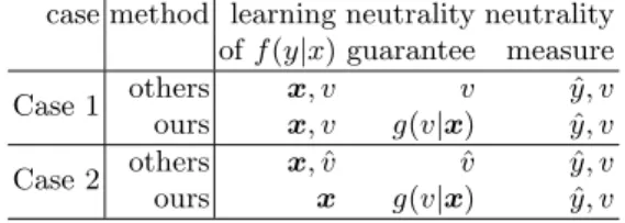
The values used for the learning of f (y | x), the guarantee of neutrality, and the measurement of neutrality are summarized in Table 3. For the guarantee of neutrality, we consider the following two cases.
Case 1 assumes that the values of the viewpoint random variable are provided in examples. In this case, our method performs neutralization with respect to the model of the viewpoint learned from the examples, whereas other methods perform neutralization with respect to the actual viewpoint values provided.
Case 2 assumes that the values of the viewpoint are not provided. Instead, the model of the viewpoint variable, g(v |x ), is provided. In this case, our method again learns the model of the target without using values of the viewpoint and performs neutralization with respect to the given model g. Other methods need the values of the viewpoint, so these are estimated as ˆ v = argmax v g(v |x ). Other methods then learn the model of the target with (x, v), and neutralization is ˆ performed with respect to ˆ v.
As a measurement of neutrality, all methods used the true viewpoint value v in both cases.
Results. Figure 1 shows the experimental results. In the graphs, the best result is at the left top. Comparing the results of NB and NBns in Case 1, we can see that the improvement of neutrality by elimination of the viewpoint variable is limited. The same applies to LR and LRns.
In Case 1, CV2NB achieves a neutrality of nearly 0 in terms of both NPI and ˆ η in both datasets. In addition, the decrease in the accuracy of the prediction is less than 1% in the Adult dataset and 5% in the Dutch Census. Thus, neutralization by CV2NB works successfully in Case 1. On the other hand, neutralization by CV2NB does not work well in Case 2; the neutralization level is almost the same as it is for NBns. CV2NB modifies the target prediction model so that the CV score with respect to the given examples becomes zero. This can cause the prediction model to overfit the given examples. Hence, the NPI and ˆ η of CV2NB with respect to the unseen values of the viewpoint are large, as seen in the results of Case 2.
In Case 1, PR successfully balances the NPI and the accuracy for the Adult
dataset, but it fails to balance the accuracy and ˆ η. This is because NPI evaluates
Table 3. Summary of the treatment of the viewpoint random variables in two settings case method learning neutrality neutrality
of f(y|x) guarantee measure
Case 1 others x, v v y, v ˆ
ours x, v g(v|x) y, v ˆ Case 2 others x, v ˆ ˆ v y, v ˆ
ours x g(v|x ) y, v ˆ
neutrality with respect to the average of the given examples, while ˆ η evaluates the lowest neutrality for all values of y and v as the worst case. This result indicates that the dependency of the predictions of target Y to the predictions of viewpoint V can be strong for some y and v, even when the NPI is kept small.
In Case 2, neutralization with PR did not work well in either dataset. This was again due to overfitting; this can be confirmed by the fact that the NPI of v and y is large in Case 2 even when the NPI of ˆ v and y is kept small (these results are omitted due to space limitations).
In both cases, our proposal, VN, successfully balances neutralization and accu- racy of the predication by changing η. Furthermore, the decrease in the accuracy of the prediction was at most 5%, even after strong neutralization with small η.
In some cases, the accuracy of VN becomes unstable with small η. The reason is thought to be the nonconvexity of the neutrality constraint. VN always guaran- tees neutrality of the prediction model, but the accuracy of the prediction can suddenly drop if the solution is captured by a local optimum.
5.2 Regression
Settings. In order to investigate the behaviors of neutralization in linear regres- sion, we performed experiments of η-neutral linear regression with the Housing dataset [5]. This dataset contains 506 examples with 14 attributes; the MEDV (median value of owner-occupied homes, in $1000s) and the LSTAT (% lower status of the population ) were used as the target and viewpoint values, respec- tively. Letting the regression parameters of the target f and viewpoint g be w and w v , respectively, the predicted values were ˆ y = w T x and ˆ v = w T v x . The ac- curacy of the prediction was measured by the root-mean-square error (RMSE), and ˆ η was used as the measure of neutrality.
Results. Figure 2 shows the scatter plots of (ˆ y, y) (the top row) and (ˆ y, ˆ v) (the bottom row). From left to right, the neutrality parameter η was varied as η ∈ { 1.0, 3.0, 10.0 } . The (ˆ y, v) plot represents the prediction accuracy of the ˆ regression model. When the model achieves a better RMSE, the points in the (ˆ y, y) plot concentrate more along the diagonal line. At the same time, the (ˆ y, ˆ v) plot represents neutrality. If the neutrality is low, any correlation between ˆ y and ˆ
v appears in the (ˆ y, v) plot. ˆ
In Figure 2 (h), a strong negative correlation between ˆ y and ˆ v can be found.
Thus, this regression model has a low neutrality if no neutralization is performed.
PR VN
CV2NB
LRLRns
NBns NB
(a) NPI, Adult, Case 1
CV2NB NBNBns PR LRLRns VN
(b) NPI, Adult, Case 2
PR LR LRns
CV2NB
NB NBns
VN
(c) NPI, Dutch Census, Case 1
CV2NB NBNBns
PR LRLRns
VN
(d) NPI, Dutch Census, Case 2
PR VN
CV2NB
LRLRns
NBns NB
(e) ˆ η, Adult, Case 1
PR VN
CV2NB LRLRns
NBNBns
(f) ˆ η, Adult, Case 2
PR LR LRns
CV2NB
NB NBns
VN
(g) ˆ η, Dutch Census, Case 1
CV2NB NBNBns
PR LRLRns
VN