- 122 - IEEE Workshop on Nonlinear Circuit NetworksDecember 9-10, 2011

Analysis of Simple Stochastic Resonance with Various Noise Levels

Shota Ozaki

Dept. of Telecommunications, Kagawa National College of Technology

Email: [email protected]

Shintaro Arai

Dept. of Communication Network Eng., Kagawa National College of Technology

Email: [email protected]

Takaya Yamazato Inst. of Leberal Arts & Sciences,

Nagoya University

Email: [email protected] Yoshifumi Nishio

Dept. of Electrical and Electronic Eng., Tokushima University

Email: [email protected]

Abstract—In this paper, we analyze two simple stochastic

resonances with various noise levels. First, it is analyzed that SR in a double-well potential which is well-known as a typical bistable SR model. Second, we add a one dimension to the bistable SR model and increase two stable states to the model, namely, the system is extended to “four-stable state”. Using these SR models, we carry out computer simulations and analyze the state of SR when the intensity of the noise is changed.

I. I

Stochastic resonance (SR) is a nonlinear phenomenon in which a responsiveness of a system is improved by adding suitable noise to certain nonlinear systems. Recently, SR has attracted a great deal of attention from a variety of researchers, including nonlinear circuits and systems, semiconductor de- vices and biology[1]–[5]. In this paper, we consider that SR is applied to a communication system which is one of engineering systems. In standard communication systems, the signal detection becomes difficult according to increase a noise level. We expect that it is possible to detect the signal, which is influenced significantly by noise, by applying SR to the communication systems. For robustly detecting the signal in the communication system using SR, a control of SR by noise is very important task. Therefore, we consider that it is necessary to investigate a relationship between SR and noise.

Based on the above research background, this paper focuses on an analysis of SR with various noise levels using simple SR model. First, we analyze SR in a double-well potential which is well-known as a typical bistable SR model. The bistable system has two stable states (+1 or − 1). Thus, we can regard the two stable states as 1bit data in the communication systems. Next, we add a one dimension to the bistable SR model and increase two stable states to the model, namely, the system is extended to “four-stable state”. In this paper, we call the extended SR model “SR in a quadruple-well potential”.

Here, four-stable states of the extended system are ( − 1, − 1), (+1, − 1), ( − 1, +1) and (+1, +1). Thus, we can regard the two stable states as 2bit data in the communication systems.

This paper describes an outline of SR in the quadruple-well

U(x) U(x)

U(x) U(x)

x x

x x

t1 t2

t3 t4

(a) (b)

(d) (c)

State of x

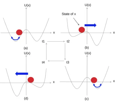
Fig. 1. Mechanism of SR in bistable system.

potential. In addition, we carry out computer simulations and analyze the state of SR when the intensity of the noise is changed.

II. SR

-

Here, we briefly explain SR in the double-well potential. In Ref. [5], the bistable SR is performed by following equations

dx

dt = f (x) + Dn(t) + s(t) (1) s(t) = A sin(2πf

t) (2) f (x) = − dU

(x)

dx (3)

U

(x) = − 1 2 x

+ 1

4 x

(4)

Where U

(x) is a bistable potential having two local mini- mums, x is a state variable, s(t) is an input signal, A is an

- 122 -

IEEE Workshop on Nonlinear Circuit Networks December 9-10, 2011

x

A B

C D

y State

(x, y)

+1 -1

+1

-1

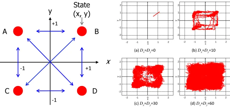
Fig. 2. Four-ideal-stable states.

amplitude of the input signal, n is assumed to be the additive white Gaussian noise AWGN, D is an intensity of noise. An effective potential U (x, t) is described as follows.

U (x, t) = U

(x) + xs(t)

= − 1 2 x

+ 1

4 x

+ xA sin(2πf

t) (5) Figure 1 shows a mechanism of SR in the bistable system.

III. SR

-

In this study, we add a new state variable “y” to this bistable system and extend the system to SR in the quadruple-well potential. First, based on Eq. (1), the equation of the state x is described as follows.

dx

dt = f (x) + D

n

(t) + s(t) (6) Where n

is noise added to the state x, D

is an intensity of noise for the state x. Next, the equation of the new state y is described as follows.

dy

dt = f (y) + D

n

(t) + s(t) (7) f (y) = − dU

(y)

dy (8)

U

(y) = − 1 2 y

+ 1

4 y

(9)

Where n

is noise added to the state y, D

is an intensity of noise for the state y. In this study, n

and n

are assumed to be (AWGN). Additionally, the values of n

and n

are different from each other. In other words, the n

and n

are independent of each other.

(a) D

= D

=0

-2 -1 0 1 2

-2 -1 0 1 2

y

x 1 2

y

x

(b) D

= D

=10

-2 -1 0 1 2

-2 -1 0

(c) D

= D

=30

-2 -1 0 1 2

-2 -1 0 1 2

y

x

(d) D

= D

=60

-2 -1 0 1 2

-2 -1 0 1 2

y

x

Fig. 3. Output of SR in four-stable state (Dx=Dy).

IV. S

A. Simulation conditions

Using the above system, we carry out computer simulations.

In the simulation, the two states are expressed in (x, y) planes a coordinate (point (x, y)). Figure 2 shows four-ideal-stable states of SR in the quadruple-well potential in (x, y) plane.

By changing D

and D

(i.e. noise level), we experiment to control four-stable states in this plane. As parameters of the simulation, the initial condition of x & y is “+1”, t = 100, 000.

B. Results of same noise level (Dx = Dy).

Figure 3 shows simulation results for same noise level Dx = Dy. First, in the case of D

= D

= 0 (Fig. 3(a)), we can observed that the point (x, y) centers around (+1, +1) since noise is not added to the system. Second, in the case of D

= D

= 10 (Fig. 3(b)), it can be confirmed that the point (x, y) moves the potential barrier and moves around the four-stable states. Third, in the case of D

= D

= 30 (Fig. 3(c)), the point (x, y) continually hops the potential barrier. However, we can see that the point (x, y) does not stay in one-stable state for a long time although the point (x, y) moves around the four-stable states. Finally, in the case of D

= D

= 60 (Fig. 3(d)), it can be observed that the point (x, y) move around (x, y) plane, regardless of the four-stable states.

C. Results of different noise level (fixed Dx, variable Dy).

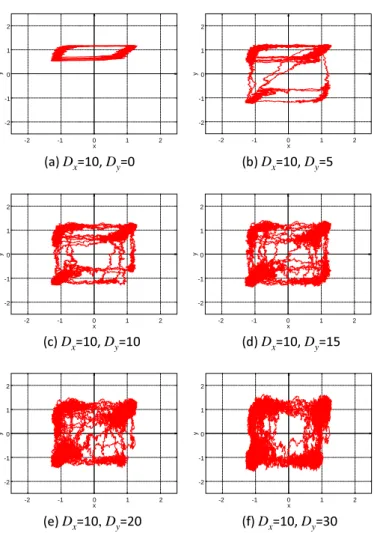
Next, Fig. 4 shows simulation results for fixed Dx = 10 and variable Dy. First, in the case of Dy = 0 (Fig. 4(a)), the point (x, y) moves a little in y-axis. On the other hands, the point hops only in x-axis. Second, in the case of Dy = 5 (Fig. 4(b)),

- 123 -

-2 -1 0 1 2

-2 -1 0 1 2

y

x

-2 -1 0 1 2

-2 -1 0 1 2

y

x

-2 -1 0 1 2

-2 -1 0 1 2

y

x

-2 -1 0 1 2

-2 -1 0 1 2

y

x

-2 -1 0 1 2

-2 -1 0 1 2

y

x

-2 -1 0 1 2

-2 -1 0 1 2

y

x

(a) D

=10, D

=0 (b) D

=10, D

=5

(c) D

=10, D

=10 (d) D

=10, D

=15

(e) D

=10 , D

=20 (f) D

=10, D

=30

Fig. 4. Output of SR in four-stable state (fixedDx, variableDy).

we can observe that the point (x, y) frequently hops in x-axis since the noise level of x (Dx) is stronger than that of y (Dy).

Third, in the case of Dy = 10 (Fig. 4(c)), the point (x, y) symmetrically hops in (x, y) plane because Dx and Dy are same values. Fourth, in the case of Dy = 15 (Fig. 4(d)) and Dy = 20 (Fig. 4(e)), we can find that the number of the point’s move increases. In other words, the point (x, y) actively hops in (x, y) plane. Finally, in the case of Dy = 30 (Fig. 4(f)), the point’s move around the origin is not confirmed in (x, y) plane. Here, we compare the results of the same noise level (Dx = Dy) and the different noise level (fixed Dx, variable Dy). By setting the different noise level, we can make the difference point’s between x-axis and y-axis and can confirm that the point move linearly. Therefore, to use the different noise levels is effective for controlling the state of the SR in the quadruple-well potential.

V. C

In this paper, we have analyzed SR in the quadruple-well potential which extended the SR in a double-well potential. As results of computer simulations, it have been confirmed that the various point’s moves by changing noise levels. However, we have performed only the qualitative analysis, such as the

behavior of the point (x, y) , in this study. Therefore, the quantitative analysis of the SR in the quadruple-well potential, such as a signal-to-noise ratio (SNR), is our future work.

R

[1] F. Chapeau-Blondeau and X. Godivier, “Theory of stochastic resonance in signal transmission by static nonlinear systems,” Physical Review E, vol. 55, no. 2, pp. 1478-1495, Feb. 1997.

[2] L. Gammaitoni, P. H¨anggi, P. Jung and F. Marchesoni, “Stochastic resonance,” Reviews of Modern Physics, vol. 70, no. 1, pp. 223-287, Feb. 1997.

[3] H. Fujisaka, T. Kamio, K. Haeiwa, “Stochastic resonance in coupled synchronization loops,” IEICE Trans. Fundamentals, vol. J90-A, no. 11, pp. 806-816, Nov. 2007. (in Japansese)

[4] A. Utagawa, T. Asai, K. Yoshida and Y. Amemiya, “Stochastic resonance in a simple electrical circuits having a double-well potential,” Technical Report of IEICE, vol. 109, no. 458, NLP2009-171, pp. 75-80, Mar. 2010.

(in Japanese)

[5] H. Nishimura, “Stochastic and Chaotic Resonances in Nonlinear Systems with Fluctuations,” J. Society of Instrument and Control Engineers, vol. 49, no. 4, pp. 244-249, Apr. 2010. (in Japanese)

- 124 -