[Paper] Adaptive Exposure-time Control Based on Image Entropy for Multiple-exposure-time Image Sensor

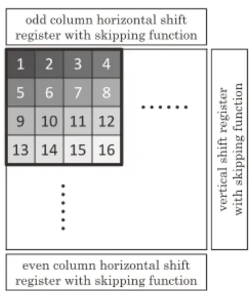
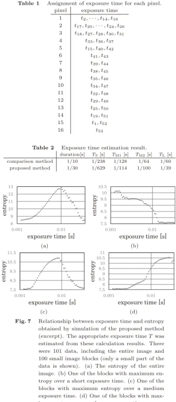
Paper. Adaptive Exposure-time Control Based on Image En-. tropy for Multiple-exposure-time Image Sensor. Kurumi Kataoka †, Yusuke Kameda (member)†, Takayuki Hamamoto (member)†. Abstract We propose an adaptive exposure-time-control method for image sensors, which can control the exposure time. for each pixel to reconstruct a high-dynamic-range image, while suppressing blown-out highlights and blocked-up shadows,. according to the luminance and contrast of the scene. First, the proposed method determines the exposure time that maxi-. mizes the entropy of the entire image, as an image with high entropy contains more object details. In order to estimate the. exposure time appropriate for the light and dark areas in the scene, the proposed method divides the image into blocks and. estimates the exposure time that maximizes the entropy for each block. Because the proposed method captures and estimates. several exposure times simultaneously, the time required for adjusting the exposure time is reduced. Simulation experiments. show the effectiveness of the proposed method.. Key words: Multiple exposure time imaging, Exposure time control, Image entropy, HDR reconstruction.. 1. Introduction. For surveillance-camera applications, high dynamic. range (HDR) images containing detailed structural in-. formation of the object, without overexposure or un-. derexposure, are required. However, in a scene with. a large difference in luminance, which exceeds the dy-. namic range (DR) of the image sensor, it may not be. possible to obtain sufficient object information owing to. insufficient or excessive exposure. Therefore, it is nec-. essary to expand the DR by applying imaging methods.. The existing method1) proposed that the image sen-. sor be equipped with a dimming filter with different. light transmittance for each pixel, to acquire images. with different exposure amounts simultaneously. A. HDR image could then be reconstructed by averaging. this acquired set of images. However, because the sensi-. tivity of the image sensor was fixed during manufactur-. ing, it was impossible to adjust the exposure amount to. an appropriate level according to the difference in the. luminance of the object. Therefore, depending on the. scene, excessive blackout or whiteout could occur, de-. teriorating the quality of the HDR image reconstructed. in the subsequent stage.. To solve this problem, an image sensor2)3) was pro-. posed that enabled multiple-exposure-time imaging,. Received August 2, 2020; Revised December 29, 2020; Accepted. March 2, 2021. †Department of Electrical Engineering, Faculty of Engineering, Tokyo University of Science. (6-3-1, Niijuku, Katsushika-ku, Tokyo 125-8585, Japan). which acquired images with different exposures, simul-. taneously, by changing the exposure time for each pixel.. In one study4), this image sensor was used to adjust the. exposure amount to an appropriate level by controlling. the exposure times according to the luminance value of. the object. This method adjusted the exposure time of. the next frame according to the imaging results of the. current frame. This process was repeated over multiple. frames. This method could, however, take some time. to determine the appropriate exposure time. Moreover,. the adjustment was not effective if the threshold value. setting was not suitable for the scene because the ad-. justment was performed based on a threshold value set. in advance.. A few studies5)7)˜9) determined the appropriate ex-. posure based on the image entropy obtained from the. imaging results. The entropy is usually large for images. with appropriate exposure containing detailed struc-. tural information of the object, but small for images. that have lost details owing to underexposure / over-. exposure, and be used to estimate the exposure time5).. The methods based on entropy were mainly intended. for imaging with a single exposure time and did not. target scenes with high contrast.. In this paper, we propose an exposure-time-control. method using an image sensor capable of capturing. multiple-exposure images for imaging a scene with. high contrast. Images with multiple exposure times. and their entropies are acquired simultaneously, and. the multiple exposure times for reconstructing a high-. ITE Trans. on MTA Vol. 9, No. 2, pp. 128-135 (2021). 128. Copyright © 2021 by ITE Transactions on Media Technology and Applications (MTA). Received October 2, 2020; Revised December 29, 2020; Accepted March 2, 2021. quality HDR image are estimated based on the values.. The entropy is calculated for each small block that con-. stitutes the image. This method can estimate the ap-. propriate exposure time for each region with different. illuminance. As much entropy as possible, of the expo-. sure time images, is acquired in a certain period; there-. fore, the exposure time can be estimated within a short. time. As a result, it is possible to perform robust ex-. posure control for changes in luminance and contrast.. In addition, when an image with high entropy is used. for HDR reconstruction, the quality of the HDR image. after reconstruction is improved10).. The proposed method estimates the exposure time. based on image entropy, which contributes to the re-. construction of high-quality HDR images in the sub-. sequent stage.This method is effective when capturing. images of a still subject without camera vibration. For. example, HDR reconstruction of images taken with the. proposed method helps to obtain high-quality photos. when shooting landscapes with a tripod. Additionally,. when a surveillance camera is used outdoors or indoors. with a single exposure time, blown-out highlights and. blocked-up shadows may occur in the image depending. on the position of the light source. These areas may. contain information about suspicious persons and ob-. jects. In addition, the brightness of the subject and the. presence or absence of shadows change depending on. the changing altitude of the sun and on whether the. lighting is turning on or off. By reconstructing im-. ages whose exposures are properly controlled by the. proposed method, overexposure / underexposure can. be suppressed adaptively in response to changes in il-. luminance. This is effective for detecting abnormalities. with a surveillance camera for security and traffic ap-. plications. This method could also be used in industrial. cameras for identifying and observing objects.. 2. Proposed exposure-time-control method. In the proposed exposure-time-control method, we. use a multiple-exposure-time image sensor. Figure 1. shows this image sensor2)3). This image sensor can con-. trol the reset and readout phases of the charge stored in. a photodiode in units of up to 4 4 pixel blocks. The. control in block units is realized by using the skipping. selection and reset functions of the vertical/horizontal. scanning circuits.. 2. 1 Multiple-exposure-time imaging method. Figure 2 shows the exposure timing. In order to cap-. ture an image with an appropriate exposure in a sit-. even column horizontal shift register with skipping function. odd column horizontal shift register with skipping function. ve rt. ic al. sh ift. re gi. st er. w ith. sk ip. pi ng. fu nc. tio n. 1 2 3 4. 5 6 7 8. 9 10 11 12. 13 14 15 16. Fig. 1 Imaging surface of the image sensor2) that con-. trols the phase of charge reset and readout in. units of 4 × 4 pixel blocks. Images can be captured simultaneously and independently, with up. to 16 different exposure times.. time. ImagingEstimation of Exposure Times. 1. 2. 15. 16. 1. 2. 3. 4. Fig. 2 Exposure timing and exposure time of each pixel. in the proposed method. tk represents the n. types of exposure time that exist between t1 and. tn, which are evenly determined by the ratio r.. Using these n types of exposure-time images as. samples, the exposure time during the imaging. period is estimated. T represents the four types. of exposure times determined. Pixels other than. the 16th pixel, to which the exposure time tn is. assigned, are exposed multiple times; all imag-. ing at t1, t2, · · · , tn is completed while imaging tn. A finite amount of time is required for the. sensor to reset and read the accumulated charge,. but this time duration is ignored here.. (a) 4 4 (b) 2 2. Fig. 3 (a) and (b) are the exposure-time-control pat-. terns for the exposure time estimation period. and imaging period, respectively. The resolution. of (a) is 1/4 of that of (b).. uation where the luminance and contrast change over. time, two periods are introduced: the exposure-time-. estimation period for estimating the appropriate expo-. sure times and the imaging period for imaging with the. estimated exposure times. The estimation period can. be set according to the changes in the imaging environ-. ment.. In the exposure-time-estimation period, the entropies. 129. Paper » Adaptive Exposure-time Control Based on Image Entropy for Mmultiple-exposure-time Image Sensor. of various exposure time images are acquired in order. to estimate the appropriate exposure time. Images are. taken with as many different exposure times as possi-. ble for accurate estimation. Therefore, the exposure. of an image sensor capable of capturing multiple expo-. sure times is controlled in units of 4 × 4 pixel blocks (Fig.3(a)), and it is possible to capture images with 16. different exposure times simultaneously. The exposure. timing is determined so that these 16 types of pixels. can be utilized fully.. The shortest exposure time within the exposure-time-. estimation period is t1 and the longest exposure time is. tn. For simplicity, the time required to reset and read. the accumulated charge is ignored. We determine the. exposure time and timing so that n types of exposure-. time images from t1 to tn can be acquired by the time. imaging with the longest exposure time tn has been. completed. For this purpose, the sum of the exposure. times read by each of the 16 pixels must be tn. When. images with n types of exposure times are captured,. the sum of these exposure times should be within 16tn.. Therefore, if the ratio of the exposure time to be imaged. is r, it can be expressed as tk = t1r k−1(1 < k <= n) such. that t1 + t2 + · · ·+ tn <= 16tn; that is, the maximum n that satisfies t1+ t1r. 1+ · · ·+ t1rn−1 <= 16t1rn−1 can be calculated. This determines the exposure times tk and. ratio r used for estimation.. Each exposure time is set such that imaging with n. types of exposure times is completed in the period un-. til the end of imaging with exposure time tn. We are. not concerned here with read time. n types of expo-. sure time are assigned to 16 types of pixels so that the. sum of the exposure times of each pixel is within tn.. This sensor can only capture with 16 different, simulta-. neous exposure times. However, by setting a different. exposure time again for the pixels that have finished ac-. cumulating charges, it is possible to acquire n types of. exposure-time images before imaging with the longest. exposure time tn has been completed. For instance, as. shown in Fig. 2, one pixel takes an image with only an. exposure time of tn while another pixel is exposed with. a slightly shorter time than tn and then sets a very short. exposure time. Ignoring the readout time, this pixel can. capture two different exposure time images. Similarly,. we combine the n types of exposure times obtained so. that the sum is tn or less, and assign them to 16 pixels. each. As described above, the exposure timing within. the exposure time estimation period is determined.. During the imaging period, the exposure of an im-. age sensor capable of multiple-exposure-time imaging. is controlled in units of 2 × 2 pixel blocks (Fig.3(b)) in order to suppress the decrease in spatial resolution.. Imaging is performed with four types of exposure times. determined by the exposure-time-estimation period.. 2. 2 Determining exposure time based on en-. tropy. The entropy of the image captured during the. exposure-time-estimation period is used to determine. the appropriate exposure time during the exposure pe-. riod. Normally, the entropy of an image is calculated. from the luminance value, as shown in Eq.(1)6).. E = L−1∑. l=0. −P (l) · logP (l) (1). P (l) = H(l). N (2). L is the number of gradations of the image, H(l) is. the number of pixels of the luminance value l, and N. is the total number of pixels of the image. An image. with an appropriate exposure, which contains many de-. tails of the object, has a large entropy because the his-. togram bias is small. On the other hand, in an image in. which the structural information of the object has been. lost because of blackout/whiteout, the entropy becomes. small because the histogram is largely biased. By using. this characteristic, it is possible to estimate an appro-. priate exposure time5).. ( 1 ) Middle exposure time 1. The middle-exposure-time image is captured for ac-. quiring more information in the medium luminance re-. gion that is dominant in the scene. Therefore, the. medium exposure time during the imaging period is. determined based on the entropy calculated using the. histogram of the entire image. The entropy of each of. the n types of exposure-time images acquired during. the exposure-time estimation period is calculated from. Eq.(1). Then, as shown in Fig.4, the exposure time of. the image with the maximum entropy can be estimated.. Let this exposure time be the medium exposure time. TM1 in the imaging period.. ( 2 ) Determining short / long exposure time. In the proposed method, the short / long exposure. time of the imaging period is determined based on the. entropy of the high / low luminance region.. The image is divided into m blocks based on the as-. sumption that the high and low-luminance regions ex-. ist locally. Then, a block in which the high/low lu-. minance region occupies a large proportion can be ob-. ITE Trans. on MTA Vol. 9, No. 2 (2021). 130. en tr. op y. exposure time. middle exposure time. max. Fig. 4 Determination of medium exposure time, using. entropy.. block1 block2. block3 block4 n (a) Example of different exposure time images after block division. (m = 4). max. en tr. op y. exposure time. block1. (b)Block 1 with medium. luminance. mmax. en tr. op y. exposure time. block2. (c)Block 2 containing. high-luminance area. max. en tr. op y. exposure time. block3. (d)Block 3 containing. high-luminance area. max. en tr. op y. exposure time. block4. (e)Block 4 containing. low-luminance area. Fig. 5 Determination of short / long exposure times. by entropy for each block. Among the exposure. times T1 to T4, where the entropy is the maxi-. mum in each block, the shortest and longest ones. are the short exposure time TS and long expo-. sure time TL, respectively.. tained. We estimate the exposure times suitable for. these blocks by calculating the entropy for each block. using Eq.(1). Figure 5 shows an example of acquiring n. types of exposure-time images during the exposure time. estimation period and dividing them into m blocks. As. shown in Fig. 5, the exposure time at which the max-. imum entropy is obtained differs from block to block.. The block with the shortest exposure time, which has. the maximum entropy, is considered to be occupied. by the high-luminance region. This exposure time is. adopted as the short exposure time TS of the imaging. period. Similarly, the block with the longest exposure. time, which has the maximum entropy, is considered to. be occupied by the low-luminance region. This expo-. sure time is adopted as the long exposure time TL of. the imaging period.. ( 3 ) Middle exposure time 2. In the proposed method, in order to acquire more ob-. ject information, another middle exposure time is set,. in addition to TM1. This second middle exposure time. is called TM2. First, we use the information on the ex-. posure time that maximizes the entropy in each block. constituting the image, in Section 2.2.(2). We count. how many blocks maximize the entropy for each expo-. sure time. Next, we investigate which of the already. determined TS-TM1 or TM1-TL has the larger number. of exposure time samples included in that section. As. shown in Fig. 6, TM2 is the time when the number of. blocks with the maximum entropy is the largest among. the exposure times existing in the section with a larger. number of samples. If TM2 is shorter than TM1, the. shorter exposure time is TM1 and the longer exposure. time is TM2. N. um be. r o f b. lo ck. s w. ith m. ax im. um e. nt ro. py. exposure time middle exposure time. Fig. 6 Determining the second medium exposure time. (example of m = 100, n = 53). The second. medium exposure time TM2 has the largest num-. ber of blocks with the maximum entropy in the. period with a large number of samples when di-. vided by the first medium exposure time TM1.. Depending on the number of image divisions,. TM1 estimated from the entropy of the entire im-. age may not correspond to the largest number of. blocks.. 3. Performance evaluation by simulation. 3. 1 Evaluation method. A simulation was performed to confirm the effective-. ness of the proposed method in a scene with a large. difference in luminance. Using a Canon EOS 50D, 37. images were captured with the exposure time changed. from 1/810 to 1/30 s. For images with different expo-. sure times, images with arbitrary exposure times were. created by estimating the relationship between the ex-. posure time and brightness value for each pixel. After. 131. Paper » Adaptive Exposure-time Control Based on Image Entropy for Mmultiple-exposure-time Image Sensor. that, noise was added and reduced according to the. pixel block that controlled the spatial resolution. In. this way, the image taken by the image sensor2) capa-. ble of taking multiple exposure times was reproduced. and used for the simulation.The size of the images was. 1588× 2385, and the number of bits of the image data was 16-bits. The images in this paper were changed to. 8-bit. In the simulation, t1 was set to 1/810 s, tn was. set to 1/30 s, and the number of block divisions m was. set to 100. From these t1 and tn, r = 1.0654 and n = 53. were calculated, and an image of the frame for estimat-. ing the exposure time was created. Table 1 shows how. n different exposure times were specifically assigned to. 16 different pixels in this simulation.. The conventional method4) was used for comparison.. In this method4), the presence or absence of overexpo-. sure or underexposure of the initial exposure time ac-. quired by multiple-exposure-time imaging was judged. by the brightness value of the pixel. When the ratio. of the number of overexposed / underexposed pixels to. the entire image was higher than a threshold value, the. shortest and longest exposure times were determined. by repeating the process of halving or doubling the ex-. posure time. The parameters used in the comparison. method were the initial exposure time of 1/30 s, black-. out judgment brightness value of 50, whiteout judgment. brightness value of 200, and blackout / whiteout thresh-. old value of 10 % of the total number of pixels.. In this simulation, the time required to determine. the appropriate exposure time was compared with the. image quality of each exposure time taken with the es-. timated exposure time. In addition, as HDR image re-. construction is expected to be the main application des-. tination, image quality comparison was also performed. when the images captured by the comparison method. and proposed method were HDR reconstructed by the. method1).. 3. 2 Evaluation results. Figure 7 shows the relationship between exposure. time and entropy in the simulation of the proposed. method. 101 data were used for the estimation, includ-. ing the entire image and 100 blocks, so that only a part. of the data was extracted. Images of the exposure time. determined by each method are shown in Figures 8 and. 9. Table 2 shows the determined exposure time and. the estimated time required to determine the exposure. time.. As shown in Figures 8 and 9, in the comparison. method4), a large amount of overexposure occurred near. Table 1 Assignment of exposure time for each pixel.. pixel exposure time. 1 t2, · · · , t14, t16 2 t17, t20, · · · , t24, t26 3 t18, t27, t28, t30, t31. 4 t33, t36, t37. 5 t15, t40, t42. 6 t41, t43. 7 t39, t44. 8 t38, t45. 9 t35, t46. 10 t34, t47. 11 t32, t48. 12 t29, t49. 13 t25, t50. 14 t19, t51. 15 t1, t52. 16 t53. Table 2 Exposure time estimation result. duration[s] TS [s] TM1 [s] TM2 [s] TL [s]. comparison method 1/10 1/238 1/128 1/64 1/60. proposed method 1/30 1/629 1/114 1/100 1/39. 8 9. 10 11 12 13. 0.001 0.01. en tr. op y. exposure time [s] (a). 7.5 8. 8.5 9. 9.5 10. 10.5. 0.001 0.01. en tr. op y. exposure time [s] (b). 7.5. 8.5. 9.5. 10.5. 11.5. 0.001 0.01. en tr. op y. exposure time [s] (c). 7.5 8. 8.5 9. 9.5 10. 10.5 11. 0.001 0.01. en tr. op y. exposure time [s] (d). Fig. 7 Relationship between exposure time and entropy. obtained by simulation of the proposed method. (excerpt). The appropriate exposure time T was. estimated from these calculation results. There. were 101 data, including the entire image and. 100 small image blocks (only a small part of the. data is shown). (a) The entropy of the entire. image. (b) One of the blocks with maximum en-. tropy over a short exposure time. (c) One of the. blocks with maximum entropy over a medium. exposure time. (d) One of the blocks with max-. imum entropy over a long exposure time.. the light bulb, which was the high-luminance area at. the lower left of the short-exposure-time image. On. the other hand, the proposed method had less overex-. posure, and the information on the wall surface of the. box in which the light bulb was attached could be ob-. tained. In addition, as shown in Table 2, the compari-. son method took 1/10 s to estimate the exposure time.. On the other hand, the proposed method completed the. estimation in 1/30 s. It can be seen that the proposed. method could estimate an appropriate exposure time. in a shorter time than the compared method. There-. ITE Trans. on MTA Vol. 9, No. 2 (2021). 132. (a) Imaging with TS (b) Enlarged view of (a). (c) Imaging with TM1 (d) Imaging with TM2. (e) Imaging with TL. Fig. 8 Imaging result of comparison method4).. (a) Imaging with TS (b) Enlarged view of (a). (c) Imaging with TM1 (d) Imaging with TM2. (e) Imaging with TL. Fig. 9 Imaging results of the proposed method.. fore, it could be confirmed that the proposed method. could follow sudden changes in illuminance and bright-. ness difference and was a more robust exposure-control. method.. Furthermore, HDR reconstruction processing1) by ad-. dition averaging was performed using four exposure. time images acquired by the comparison method and. proposed method. The results are shown in Figures. (a) HDR reconstructed image (b) High-luminance area. Brightness value. N um. be r o. f p ix. el s. (c) Histogram of (a). Fig. 10 HDR reconstruction result of comparison. method4).. (a) HDR reconstructed image (b) High-luminance area. N um. be r o. f p ix. el s. Brightness value (c) Histogram of (a). Fig. 11 HDR reconstruction result of the proposed. method.. 10 and 11. From Figures 10 and 11, in the compar-. ison method4), overexposure occurred near the light. bulb in the high-illuminance region even after HDR re-. construction. On the other hand, it can be seen that. the proposed method suppressed overexposure. In ad-. dition, from the histograms in Figures 10 (c) and 11. (c), it can be seen that the proposed method had a. wider range of brightness values than the comparison. method4). Therefore, it could be confirmed that overex-. posure and underexposure were suppressed by enlarging. the DR and that the proposed method contributed to. improving the quality of the HDR image reconstructed. in the subsequent stage.. 133. Paper » Adaptive Exposure-time Control Based on Image Entropy for Mmultiple-exposure-time Image Sensor. 4. Conclusions and future works. In this paper, we proposed an exposure-time-control. method based on image entropy that was adaptive to. the luminance of objects, for an image sensor capable of. capturing multiple exposure times. The effectiveness of. the proposed method was demonstrated through simu-. lations.. The future task will be to implement the hardware. for the proposed method and verify the working of ac-. tual machine. In this paper, the readout speed for the. image sensor is not considered for the sake of simplic-. ity. When implementing the proposed method with a. multiple-exposure-time image sensor, it is necessary to. determine the exposure timing in consideration of the. readout time. Specifically, it is conceivable to prevent. the short-time readout from being repeated in a spe-. cific pixel or to reduce the number of exposure times. acquired during the exposure time estimation period.. Even if each pixel is exposed only once and the type. of exposure time is n = 16, the proposed method still. works effectively. Even so, the larger the value of n, the. more accurate the estimation. In future work, it will be. necessary to carefully consider the effect of the value of. n on the estimation result.. Additionally, in this proposal, it cannot be said that. the number of image divisions m and its effect on the. estimation result was sufficiently examined. Since the. exposure time that maximizes the entropy is obtained. for each block and the shortest and longest are ulti-. mately selected, dividing the high-light / low-light re-. gions into multiple parts poses no problems. Rather,. in order to create a small image block in which the. high-light / low-light regions occupy most of the area,. it is better to divide the image into small blocks, but. if the image is divided into many blocks, the amount. of calculations necessary increases. If the block size is. reduced to about several pixels, the influence of noise. becomes large, and it becomes difficult to observe the. fluctuation of entropy with exposure time. At present,. the number of blocks m=100 is determined by consid-. ering that the areas smaller than 1% of the image are. unlikely to be regions of interest. The other reason for. the chosen value of m is that the 1/100 size of the image. used in this evaluation experiment is not small enough. to be significantly affected by noise. In the future, it. will be necessary to consider a more appropriate block. size.. Furthermore, in this simulation, the estimated time. does not include the time required for calculation. The. proposed method takes about 40 seconds to process. n = 53 images. The conventional method takes about. 7 seconds. These values are the times required for the. simulations alone, so the actual processing speed of the. sensor needs to be considered separately. In order to. use the proposed method over a short time, even with. actual sensors, the entropy calculation and the feed-. back of the exposure setting should be done over a short. time. Currently, we calculate the entropy in the usual. way to achieve accurate estimation, but we would like. to consider shortening the processing time required by. reducing n, accelerating the calculations, or using ap-. proximate calculations.. In future work, we will also examine an exposure-. time-estimation method that is suitable for moving ob-. jects.. Acknowledgments. This work was supported by JSPS KAKENHI Grant. Number JP20K19829.. References. 1) S. K. Nayar and T. Mitsunaga : “High Dynamic Range Imag-. ing: Spatially Varying Pixel Exposures”, Proceedings IEEE. Computer Society Conference on Computer Vision and Pat-. tern Recognition, 1, pp. 472-479 (Feb. 2000). 2) T. Kobayashi, Y. Miyamoto and T. Hamamoto : “Interleave-. Integration-Control Image Sensor”, The Seventh International. Workshop on Image Media Quality and its Applications, pp.. 21-24 (2014). 3) T. Yamazaki, T. Otaka and T. Hamamoto : “Spatiotempo-. rally Varying Imaging Method for Dynamic Range, Temporal. Resolution and SNR Improvement , Journal of The Insti-. tute of Image Information and Television Engineers, 69, 3, pp.. J106-J112 (Feb. 2015). 4) T. Kosaka, T. Kobayashi and T. Hamamoto : “Light-adaptive. Imaging Method using Interleave-exposure-control Image Sen-. sor (in Japanese)”, ITE Technical Report, 40, 15, pp. 21-24. (2016). 5) M. T. Rahman, N. Kehtarnavaz and Q. R. Razlighi : “Us-. ing Image Entropy Maximum for Auto Exposure”, Journal of. Electronic Imaging, 20, 1, pp. 1-10 (2011). 6) J. Ning, T. Lu, L. Liu, L. Guo and X. Jin : “The Optimization. and Design of the Auto-exposure Algorithm Based on Image. Entropy”, 2015 8th International Congress on Image and Sig-. nal Processing, pp. 1020-1025 (Oct. 14-16, 2015). 7) N. Kehtarnavaz and M. T. Rahman : “Adaptive Automatic. Exposure Apparatus and Method for Digital Images , U. S.. Patent US8743235B2 (Jun. 3, 2014). ITE Trans. on MTA Vol. 9, No. 2 (2021). 134. 8) Z. Chen, Y. Chen, D. Khosla and D. J. VanBuer : “Real-. time Auto Exposure Adjustment of Camera using Contrast. Entropy”, U. S. Patent US9894285B1 (Feb. 13, 2018). 9) J. Kim, Y. Cho and A. Kim : “Exposure Control Using. Bayesian Optimization Based on Entropy Weighted Image. Gradient”, 2018 IEEE International Conference on Robotics. and Automation (ICRA), pp. 857-864 (May 21-25, 2018). 10) R. Pourreza-Shahri and N. Kehtarnavaz : “Automatic Ex-. posure Selection for High Dynamic Range Photography”,. 2015 IEEE International Conference on Consumer Electron-. ics (ICCE), pp. 471-472 (Jan. 9-12, 2015). Kurumi Kataoka received her B.S. degree in Electrical Engineering from the Tokyo Uni- versity of Science, Tokyo, Japan, in 2020, and is currently a masters student. Her research interests include image processing and imaging devices.. Yusuke Kameda received his B.E., M.E., and Ph.D. degrees in Engineering from Chiba Uni- versity, in 2006, 2008, and 2012, respectively. He is currently a Junior Associate Professor with the De- partment of Electrical Engineering at Tokyo Uni- versity of Science. His research interests include computer vision and video coding.. Takayuki Hamamoto received his B.S. and M.S. degrees from the Tokyo University of Sci- ence (TUS), Tokyo, Japan, in 1992 and 1994, respectively, and the Dr. Eng. degree from the Uni- versity of Tokyo, Tokyo, Japan, in 1997, all in Elec- trical Engineering. He is currently a Professor with the Department of Electrical Engineering, TUS. His current research interests include image processing, computer vision, and computational image sensors.. 135. Paper » Adaptive Exposure-time Control Based on Image Entropy for Mmultiple-exposure-time Image Sensor