(1.2) IA!fr+pt!fr=O, in sii, (W=O, on L

NUMERICAL ASYMPTOTIC STABILITY OF THE FINITE ELEMENT SCHEME FOR A SYSTEM OF NONLINEAR

PARABOLIC EQUATIONS ARISING IN CHEMICAL REACTIONS

By Kazuo IsHIHARA

(Received Nov. 14, 1983)

1. Introduction

This paper is concerned with the finite element solutions of the initial boundary value problem for the system of nonlinear parabolic equations:

(1.1)

== dl Zlu -- blunivn2, xE 9, tÅr O, 0u _ot

== d2Av- b2untvn2, xG 9, tÅr O, Ov _at

u(x, t)==O, v(x, t)==O, xGL tÅrO,

u(x, O) :uo(x), v(x, O)=vo(x), xG9.

Here x =(xi, x2,..., x.), 9 is a bounded convex domain in the n-dimensional Euclidean

n

space R", the boundary T of 9 is piecewise smooth, A js the Laplace operator (A == 2 02/

i= 1

Ox7• ), ni, n2 are positive integers, di, d2, bi, b2 are positiVe constants, and given functions

uo(x), vo(x) are continuous and nonnegative, and uo(x), vo(x) satisfy the boundary conditions. Systems of this type arise, for example, in chemical engineering [4, 12, 14, 15]. In such cases, u,v represent the chemical concentrations, so that u, v are required to be nonnegative. Pao [14] established the uniqueness, existence and asymptoticbehavior forthe nonnegative solution {u(x, t), v(x, t)} of (1.1), and showed that there exist positive constants ri, r2 such that

O5 u(x, t) S r, exp ( --- di ptit), O S. v(pe, t) S r2 exp (- d2"i t), xe si, tÅr O,

where pti ÅrO is the least eigenvalue of the eigenvalue problem

(1.2) IA!fr+pt!fr=O, in sii,

(W=O, on L

2 Kazuo lsHiHARA

Recently, the finite element method has become more wjdely recognized as one of the most powerfu1 methods for obtaining numerical solutions of the initial boundary value problems. In [1, 7, 17], it is shown that the finite element solution converges to the exact solution for a single equatien of parabolic type.

The aim of this paper is to study the asymptotic stability of numerical solutions for (1.1). We can show that the asymptotic behavior of the finite element solution is similar to the one of the continuous problem, under appropriate assumptions. Finally, a nu- merical example is given to indicate the validity of our results.

For the finite element approximations to the Dirichlet problem of nonlinear elliptic equations, we refer to [9, 10, 11].

2. Weak form and finite element scheme

For simplicity, we assume that 2 is a polyhedral domain of R". We use the Sobolev space Hi(9) which consists of real-valued functions which together with their generalized derivatives belong to L2(9). Here L2(9) denotes the space of square integrable functions on 2. Let CO(n) be the space ofcontinuous functions on n=2ur. We also set (2. 1) Gi :: max {uo(x); xe di} ). O, G2 E max {vo(x); xe n} IO,

,r == {V e Hi(9) ; ut =O on r} ,

(ip, w)o= j.di(x)w(x)dx, a(ip, ut)= tn.,(oD.ip, , oO.ut, ),•

Now, in order to construct the finite element scheme, we introduce a weak form for (1.1) in the following way:

Find {u(x, t), v(x, t)}eY'xV", tÅrO such that

(2.2)

(OoUt , W), +dia(u, ut)= --bi(u"iv"2, W)o forall Wec)e",

(OoVt , W),+d2a(v, W)=-b2(u"iv"2, W)o forall Weie",

u(x, O) == uo(x), v(x, O) =vo(x), xG 9.

Firstly, we triangulate the polyhedral domain 9 in such a way that n= Ti U T2 U ••• U TJ, where T,, 1SgSJ are nondegenerate closed n-simplices whose interiors are pairwise disjoint. By Pi, ISi.SN (or Pi, N+IS.i-SN+M), we denote the vertices of the tri- angulation which belong to 9 (or T). For an n-simplex T,, let P6q), PSg),...,PÅíP) be its vertices and let coSq)(x),OS.j.Sn be the barycentric coordinates of a point xET, with respect to PSq). Define

hq rdiameter of T,, h=max{h,;1$q=ÅqJ},

fi,=min {dist (PSq), the (n --- 1)-face of T, not containing PS•q)); OS.J' Åq= n}, a,= max {cos (7 tuS•g), 7caS•g)); O$iÅqj Åq= n} ,

fi = min {fi,; 1 S. qgJ}, a== max {a,; 1 S. q S. J} , with

Vcoi•g)==(0o`O.S'l) ,••., 0o`O.S.") )•

We say that a triangulation ,9-h is of acute type if a50.

Remark 1. When n=2, ,/67'h is of acute type if and only if all the angles of the tri- angles are less than or equal to z/2 [3, 6].

Further, we define the lumped mass region ca(Pi) corresponding to the vertex Pi with respect to ,9'h. The barycentric subdivision Bg• of T, corresponding to Pi which is the vertex of T, with the barycentric coordinate tuÅqoq)(x) is given by

Bg• == A {xE T,; co6q)(x)lcoS•q)(x)}•

j=1 '

Then st(Pi) is defined aS follows (see Fig. 1):

va(Pi) :v {Bg; T,E ,9"h such that Pi is a vertex of T,} .

q

t Ny -ee t N-.-- t

/l...ttt;:':vailS/i(iSi:t).:g.. /t

-r

,

t{t i tt

fttttt' i1 lh : t}ttl "s'.... :, Pi'rxh-N :,,""'tx S"Sr -- .- -! ttl

1 N. tt l i, 's.. Ae' '"

t tt ---- - ) t 'sl

I tt

Fig.1. Lumpedmassregion.

Let dii, dii, 1 S. i5N+M be the finite element basis such that (t)iG CO(si), ipi is linear on each T,,

ipi(pJ)==(61 I:ll di,(x)-(81 X.gva.((P.'])', iEi,JsN+M.

4 Kazuo lsHiHARA

Define finite element spaces which are finite dimensional subspaces as follows:

Xh == span [di- i, di-2,. . ., ip-N . .] c L2(S2) ,

Y" =span [ipt, ip2,..., ip...]cH'(S2), 7/'"={Vhe Yh; Wh=O on T}cY'.

Let Yh be the iumping operator given by

- rv+M

y,: CO(S[2)-Xh, Y,ut = 2 W(P,)di,.

i=1

By TÅrO, we denote a time increment which is pre-assigned.

We now formulate the finite element scheme for (2.1) in the following way:

Find {uh,k, vh,k}e '}eCi'hÅ~ ')ei'h at time t=kT (k=1, 2,...) such that

(2.3)

( Yh(Uh,kiUh,k-i)-, YhWh)o+dla(Uh,k-1, Wh)

=-bl((Yhuh,k-1)"i(Yhvh,k-1)"2, YhWh)o foratt WheV"h, ( :2f'h(Vh,kT-Vh,k-1) , YhWh)o +d2a(Vh,k-1, ut-h)

= -' b2((YhUh,k-i)"'(Yhvh,k-i)"2, Yhil7h)o for all Ql7hE (yfr'"h,

rv+M rv +M uh,o= 2 uo(Pi)ipi, vh,o= 2 vo(Pi)q5i•

i=1 i=1

Set

(2.4) aij----'a(ipj, dii), ISiÅq=N, 1=ÅqJ'5N+M,

(2.5) mi=(dii, dii)oÅrO, ISi5N.

If we seek the solution of (2.3) in the form

N+M N+M

u,,,= .2 C,,k(l),, v,,,== 2 4,,,ip,,

l=1 i=1

with

(i,k == Uh,k(P,), 4,,, = v,,,(P,), 1 -Åq. i .S N, lc =O, 1, 2,...,

sti,k=:4i,k=O, N+IS.iSN+M, k=O,1,2,..,,

then (2.3) may be written as

(2.6)

mi SY _{i,k -} T4 i,k"i + di ,l .N

i aii s: j, k- i = :( -- bimie Y• }k -'i 4 7• ?k -i,

miinIZ- {-ki iSt.i.E=!st,k gt,k i-+d2jN.iai,•4j,k-.t=--b2mi4/11;k-i4:•'3k-i,

forlSiÅq=N,k=1,2,..,. Here ' t,

(2•7) ei,o=uo(Pi)IO, 4i,o=vo(Pi)IO, 15iEN•

We 'note that (2.6) is the explicit scheme. • .

, In the sequel, we make the following assumptions.

Assumption 1. The triangulation ,/`7`h is of acute type.

Assumption 2. The time and space increments T, fi satisfy

IZ2 ,

OÅq T5 (n + 15 max {d,, d,} + fi2 max {biG?i-'Gg2, b2G:'Gg2-'} '

For the study of the asymptotic behavior of (2.6), we use matrix notations. Given an n' Å~ m- matrix B =(bij), BlO (or BÅrO) means that bi,-lO (or bijÅrO), 1Sign-, 1 S.jÅq.. hi.

Let Xi, 1Ei.S n- be eigenvalues of an fi Å~'i-t matrix B. The spectral 'radius ofB is defined by

p(B)=max {IAil; 1S ;S h} •

Following Ciarlet [2], an NÅ~(N+M) matrix B=(b,j) is said to be of generalized non- negative type if B has the following three properties:

(a) b,,ÅrO, b,j .S O, i i, j, 1Si Åq,. N, 1 Sj Åq,,,, N+ M, . (b) B is diagonally dominant [16, p. 23],

(c) B=:(bi,•),1;!l i, .i .;.fN is irreducibly diagonally dQminant [-16, p. 23]. '

Remark 2. Ciarlet and Raviart [3] showed that under Assumption 1, the matrix

e- aT/a:tty')'ofifh3S'dNis},ie'f,jmS'aN.i,.Iu)lmOS,(,?fi2).piiSe.Ofgeneraiizednonnegativetypetoinsurethe

We end this section by stating some general results on matrices, which are usefu1 later.

LEMMA 1 [16, p. 85]. Let B==(bi,•) be qn irreducibly diagonally dominant n-Å~n- matrix with b,iÅrO, bi,• :;O, i\j, IEI i,j-s{; fi. Then, the inverse B-i exists and B'iÅrO.

The following lemma is the Perron-Frobenius resuit.

LEMMA2 [16, p. 30]. Let B be an i-txn- matrix, Suppose either that BÅrO, or that B)O is irreducible. Then, B has a positive real eigenvalue equal to p(B), and p(B) is a simple eigenvalue of B, and to, p(B) there corresponds an eigenvector zÅrO.

in this section, we shaii inve3s`tigaAtSeY!hlPetOatsiyCmbgeoatVjicO' rbehavior of (2.6). Fof ('2.4) and

(2.5), we define matrices '

A=(a,j), 1Si,j.S..N, D=ditig(mi,•••',mN)• '

6 Kazuo lsmHARA

Consider the matrix eigenvalue problem

Since A, D are real, symmetric and positive definite, (3.1) has N positive eigenvalues OÅqZiSa2$•••:$2N and N corresponding eigenvectors yi,y2,...,yN. We begin with some lemmas.

LEMMA 3 [3, 6]. Under Assumption 1, the coejeicien ts aij, mi, I S. i .S-. N, 1 .Åq,j S.

N+M of (2.4), (2.5) satisfy

aiiÅrO, aij.SO, i#j, 1,Åq,,,i"SN, 1,Åq.,J'S.N+M, ",2:.\a,j=o, oÅq a.,fs".+.,1, lsi.sN.

LEMMA 4. Under Assumption 1, the eignevector yi of (3.1) corresponding to ZiÅrO can be chosen such that yi ==(Bi, /92,..., 6N)TÅrO, where T denotes the transpose.

PRooF. Since A is irreducibly diagonally dominant (Remark 2), we have A-iÅrO, by using Lemmas 1 and 3. Thus, A-'DÅrO. From (3.1) it fo11ows that

A-iDyi= :cl-:, yi, 1siÅq.,,,N•

Hence, an application of Lemma 2 to A- iD leads to p(A-iD) =: fi7 , y, =: (fi,,•••, B.)TÅrO•

This completes the proof.

LEMMA 5. For any positive numbers d, Z, e, it holds that dz År (1 - exp ( -- dze))le.

PRooF. By putting f(x) = x --- 1 + exp ( - x), we easily obtain

f(x)ÅrO, for xÅrO.

Thus, substituting dZeÅrO to x, we find

dzÅr(l -exp(-- dze))le. '

Therefore, the proef is complete.

LEMMA 6. Let d, e be positive constants such that

O Åq e .Åq.. fi2/(d(n + 1)). -

Sup. pose that wi,k, 15i.,Åq" N, k= OÅr 1, 2,.-.. satisfy , i -

mi Wi'k -eW i' k-1 +d jN= i aijwj,k-i S. O, IEi -S N, k= : 1, 2,••• •

Then, we have

WkOa)x ll Wfu'a)x l'l '•' ll Wftkix')lWfaka)xl''',

where

wkj.).=max {wi,j; 1Si-g N}, J' ----:O, 1, 2,....

PRooF. From Lemma 3 and the hypotheses, we get

wi,k $ wi,k- i - Sl/l- jN. i aijwJ•,k- i

= (i -- dll/zii)w,,,-,- ke j"., aijwj,k-i

jsi

S (1 '- -Sl/t j"., aij)wfuki,i) s.wfaki.i), k=:1, 2,....

Here we used the fact that 1-deaiilmiÅr.,O, -aij2-O (i \j). Therefore, Wftka)x S Wfakix '), k = 1, 2, •• •,

This completes the proof.

LEMMA 7. Let d, e be positive constants such that oÅqes fi2/(d(n + 1 )) .

For initial values wi,o, 1 S. iS. N, let {wi,k} be the solution of

mi Wi'k--eWi'k-i +djN.,iai,•wj,kdi=O, 15iS.N, k :1,2"••

Then, there exists a positive constant C such that

-C exp ( -- dAiek) S. wi,k ;.S C exp ( •-- dZiek), 1 S. i Åq.,, N, k=: O, 1,.2,... ,

where Zi ÅrO is the least eigenvalue of (3.1).

RRooF. From Lemma 4, we can choose a positive constant C such that -C6,S.w,,,SC6,, 1S.iÅq,.,IV.

Putting zi,k : wi,k - eBi exp ( --- dliek), we have

8 - KazuolsHiHARA

mi Zi'k'eZi'k-1 +djN.,1aiJ'Zj,k-1

=miWi,k--S!li,k-i +djN..iaijwj,k--i

+ (i6,m, exp (- dz,e(k -i)) (1- eXPS-L!ltl !,ie)H - dA,)

SO, ISiSN, k :1, 2,... ,

from (3.1) and Lemma 5. Thus an application,of Lemma 6 yields

max {zi,k; 1 S. i Åq= N} Emax {zi,o; 1 S. i Åq., N} S. O, k= 1, 2,... .

This implies that

wi,k S. C6i exp (- dZiek), 1 s. i Åq.,, N, k=o, 1, 2,... . Similarly, we obtain

wi,k ). -- C6i exp (- dZiek), 1 S• i Åq.., N, k= O, 1, 2,... . Therefore, by putting ,C=C max {6i; 1Si Åq= N}, we get

-- C exp (- dZtek) :.f wi,k :.f C exp ( -- dAiek), 1 S. i Åq= N, k == O, 1, 2,... .

This completes the proof.

We now have the following proposition.

PRoposiTioN 1. Under Assumptions '1 and 2, the solution of (2.6) satisLfies O-Åq--4,,,5G. OS.C,,,S.G,, 1-Åq.iÅq,,.N, k=O,1,2,....

PRooF. From (2.1), (2.7), it is clear that

OS.4,,,SG,, OS.4,,,S.G,, IS.i-SN.

Assume that

(3.2) OS.4,,j-gG,, OS.4,,j-S-;-G,, IS.i-SN, OS.J'ntSk-1,

From Assumption 2, (2.6) and (3.2), it follows that OÅqT :.f k21((n+ 1) max {di, d2}) ,

mi 4i,k -Te i, k-i + d, jN= , aisj,k -, == - b, mi4 r• lk - ,47• ?k -, E O, 1 .Åq,. i5 N,

mi gi,k '--T4 i, k-i + d2 jN.i ai,• 4j,k-1 = - b2 mi4 r• 3k -iCr• lk -i i:S O, 1 ;$ i ;:S N• , •

By applying Lemma 6 to the above equations, we obtain

(3•3) 4kk2xS-efikix"5'''S-4fiOa'xS-Gi, 4fuka'xS-4fakix"S"''S'4fiOa'xS'G2, where st .( j,). =: max {4i,j; 1 S. iS N}, 4faj.). = max {Ci,j; I S. i -S N}. Th us, from Lemma 3, Assumption 2 and (3.3), it follows that

(3.4) 1-T( d; /9i.tt +b,ci7•},--i,cr•,2,-,) ll;o, 1-T( d; 19iii + b,(g:},-,4r•i,=i,) llO•

Using (2.6), Lemma 3, (3.2),,(3.3) and (3,4), we obtain ,

G, lll 4i,, : (1 - -IIL{Stil ti --- Tb,e}i: ,=i ,4 ;•' ?, -,) ei, k-, -- [ dl ,i i2: 1 aij4j, k- i ll;; O,

jt'

G,l.ii:4,,, =(i-!dmt9.ii -Tb24r•}k-,4:•ti,=i,)4i,knyi- Tmd,2. j=N,. ai,•gj,k-iliO,

jte

for IS.iSN. Hence (3.2) holds with k--1 replaced by k. Therefore, by mathematical induction, the proof is complete.

We are now in a position to prove the main result.

THBoREM 1. Let {4i,k, 4i,k}, IS.i.S-N, k==O, 1, 2,... be the solution of (2.6). Under Assumptions 1 and 2, there exist positive constants Ci and C2 such that

O;S ei,k :S Ci exp (-diAiTk), O;:il Ci,k ::S C2 exp (- d2ZiTk), ,1 S. i Åq= N, k = O, 1, 2,... ,

where Ai ÅrO is the least eigenvalue of (3.1).

PRooF, For initial values wi,o == 4i,o, 1 ;:S i ;.S N, let wi,k be the solution of

(3.s) miWi•k-'- Yi•k-l +dljN..1ai,.wj,k-1==o, 1;:$iÅq,.N, k=l,2,,...

Put zi,k=Ci,k-wi,k. Then, from (2.6), (3.5) and Proposition 1, we have

mi Zi'k-TZi'k-i +dij".,iaijz,•,k"i=--bimi4r•3k-S73k-iSO, 1Si-SN, k=1,2,••••

Hence an application of Lemma 6 leads to

max {4i,k-wi,k; 1 S. i Åq= rv} S. max {ei,o-wi,o; 1 S. i Åq.. N} == O, k= 1, 2,,,. .

Therefore by using ProPosition 1 and Lemma 7, there exists a positjve constant Ci such that

O;-Sei,k;-Swi,k;-SCtexp(-diAiTk), 1s.i--Åq.-N, k:o,1,2,...,

where ZiÅrO is the least eigenvalue of(3.1). Similarly, there exists a positive constant C2

such that

10 Kazuo tsHiHARA

OS- C,,k S- C2 eXp ( -• d,Z,Tk), 1Si Åq.,, N, k== O, 1, 2... .

This completes the proof.

Remark 3. In [8], we showed that Zi--År"i ash.O, where Ai, pti are the least eigen- values of (3.1), (1.2), respectively.

4. Numericalexperiment

We shall show here numerical results in the two dimensional case. Let 9 be a square domain of R2 given by

9={(x, y)ER2; OÅqxÅq1, OÅqyÅq1}.

By L we denote the boundary of S2. We consider the following problem.

Problem:

OoU t ==Au--uv, in g, tÅro,

StV =Av-uv, in g, tÅro,

u:v==O, on L tÅrO,

u(x, y, O) =uo(x, y), v(x, y, O)=vo(x, y), in n.

Here

uo(x, y)=

vo(x, y) ==

y, if y.Åq-.xS.1-y, y).O, 1---x, if 1-xS.y;.Sx, x51, 1--y, if 1-ySxS.y, yS.1, x, if x;.Sy:!1-x, xi.llO, 4y-1, if yS.x;.fl-•-y, y).1!4, 3-4x, if 1-x;.Sy.Åq.,x, xÅq.,3/4, 3-4y, if 1-yi:;lxS.y, y:ll314,

4x -- 1, if x;;Sy;.Sl-- x, x).. 114,

O, otherwise.

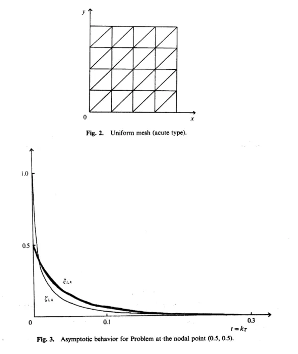
We divide 9 into uniform mesh with right isosceles triangles as shown in Fig. 2

(k=V2!8) and employ r= O.Ol, so that Assumptions 1 and 2 are satisfied. Thus, from

Theorem 1, it follows that

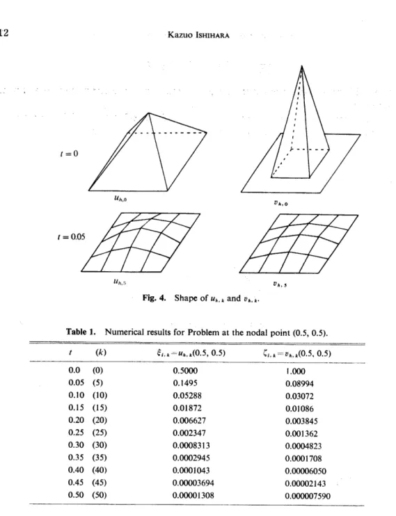
lim4,,,=:lim4,,,=:O, 1S.iÅq,,,.N.

k-co k..co

Table 1, Figures 3 and 4 present the numerical results, which demonstrate the validity of our results.

All computations were carried out on the MELcoM-CosMo 800III computer at

Kyushu Institute of Technology with the aid of single-precision arithmetic.

y

Fig. 2. Uniform mesh (acute type).

1.0

O,5

t=kT

Fig; 3. Asymptotic behavior for Problem at'the nodal point (O.5, O.S).

12 KazuolsHiHARA '

ttt

tt t ttt tttttt t t + ttt t'tt ://

Uh,O Vh,O

t = O.05

Uhvr} '' Vh,s

Fig. 4. Shape of uh,k and vh,k•

Table 1. Numerical results tor Problem at the nodal point (O.5, O.5).

t (k) 6,,,-=:-: u,,,(O.5, O.5) C,,,==- v,,,(O.5, O.5)

O.O (O) O.5000 1.000

O.05 (5) O.1495 O.08994 O.10 (10) O.05288 O.03072 O.15 (15) O.O1872 O.OI086 O.20 (20) O.oo6627 O.oo3845 O.25 (25) O.oo2347 O.oo1362 O,30 (30) O.OO08313 O.oo04823 O.35 (35) O.OO02945 O.OOO1708 O.40 (40) O.ooOI043 O.OOoo6050 O.45 (45) O.OOO03694 O.OOO02143 O,50 (50) O.OOoo1308 O.OOOO07590

References

[ 1 ] K. Baba and M. Tabata, On a conservative upwindfin(te element scheme for a convective diffusion eguaticn&H R. A, IRO Anal. Numer., 15 (1981), 3-25.- .. ',

[2] P.G. Åëiarlet, Discrete maximum principle .forfinite-dt:ffefience operator, A6qua{iones Math,, 4 (1970), 338-352.

[31 P. G, Cjarlet tn,' d P. A. Raviatt,' Maximum principle aitd, unifotm convergence for•thefinite element

method, Comput. Methods Appl. Mech. Engrg.,2(1973), 17-31.

[4] P.V.Danckwerts, Gastiquidreactions, McGraw-Hill,NewYork,1970,

[5] A, Friedman, Partiat di:fferential equations of parabolic type, Prentice-Hall, Englewood Cliffs, N. J., 1964.

[6] H. Fujii, Some remarks on ,finite element analysis of time-dependent fi'eld problems, Theory and practice in finite element structural analysis, Y. Yamada and R. H. Gallagher, ed. (1973), 91-106, Univ. of Tokyo Press.

[7] H. Fujita and A. Mizutani, On thefi'nite etement methodfbrparabolic equations, I; approximation ofholomorphic semi-groups, J. Math. Soc. Japan, 28 (1976), 749-771.

[8 ] K. Ishihara, Convergence ofthe.finite element method apptied to the eigenvalue problem au+2u==-O, Publ. Res. Inst. Math. Sci., 13 (1977), 47-60.

[9] K. Ishihara, On finite etement schemes of the Dirichtet problem for a system Qf' nontinear elli tic equations, Numer. Funct. Anal. Optim., 3 (1981), 105-136.

[10] K. Ishihara, Finite element approximations apptied to the nonlinear boundary vat"e problem au==bu2, Publ. Res. Inst. Math. Sci., 18 (1982), 17-34.

[111 K.Ishihara, Monotone explicit iterations of the finite etement approximations for the nonlinear boundary value probtem, Numer. Math. (1984 in press).

[12] C.S. Kahane, On a system of nonlinear parabolic equations arising in chemical etrgineering, J.

Math. Anal. Appl., 53 (1976), 343-358.

[131 M. Mimura, Finite di:fference methodfor a class ofsemilinearparabolic system related to physicat andbiologicalproblems, Doctoral Dissertation, Kyoto University, Kyoto, 1973.

[14] C.V.Pao, Asymptoticstabilityofacoupteddi]ffusionsystemarisingfromgas-tiquidreactions, Rocky Moutain J. Math., 12 (1982), 55-73.

[15] J. R. Pearson, Di.ffusion qfone substance into a semi-infinite medium containing another with a second order reaction, Appl. Sci. Res. Section A, 11 (1963), 321-340.

[16] R. S. Varga, Martix iterative analysis, Prentice-Hall, Englewood Cliffs, N. J., 1962.

[17] M. Zlamal, Finite etement methods.forparabotic equations, Math. Comput., 28 (1974), 393404.

Department of Mathematics, Ky"shu Institute of Technology

Note added in proof

In connection with a linear parabolic equation Oulet == ddu +f(x, t), we refer to a

forthcoming paper: K. Ishihara, On numerical asymptotic behavior of the finite element

solutionsfor parabolic equations. This paper has been accepted for publication in the

journal "Numerische Mathematik".