A trial about the evaluation of compound geophysical explorations by self‑organizing maps
著者 Yamamoto Tatsuru, Kusumi Harushige, Nakamura Makoto, Yamamoto Tsuyoshi, Tsuji Takeshi journal or
publication title
Proceeding of the 14th International Symposium on Recent Advances in Exploration Geophsics in Kyoto(RAEG2010)
year 2010‑11‑04
URL http://hdl.handle.net/10112/5638
A trial about the evaluation of compound geophysical explorations by self-organizing maps
Tatsuru YAMAMOTO1, Harushige KUSUMI 2, Makoto NAKAMURA3, Tsuyoshi YAMAMOTO4 and Takeshi TSUJI5
1 Graduate school of Kansai University
2 President, Kansai University.
3 Dept. of Faculty of Environmental and Urban Engineering, Kansai University
4 Kinki Regional Development Bureau, Ministry of Land, Infrastructure, Transport and Tourism
5 Dept. of Environment and Resource System Engineering, Kyoto University
In Japan, in the high economic growth period in 1960’s, a great number of slopes were formed to construct many roads. Now, the slopes have been aging, it is important to estimate the health of the aging slope and maintain slopes effectually. So, in situs, we usually carry out seismic wave method, surface wave method, electric method, electromagnetic wave method, frequency domain electromagnetic method and so on. However, there is not the technique to compound and interpret the result of each geophysical exploration in a numerical formula of the engineering now. Therefore, we notice to self-organizing maps (SOM) used widely in a field of the information processing engineering, and tried to interpret multidimensional data by integrating. In this paper, we classified the ground property by self-organizing maps. The classification result is relatively conformal with boring data. Therefore, it is recognized that it can be used to improve the interpretative accuracy of compound geophysical explorations. And, it can be shown that this technique is effective to estimate of the ground property of the aging slope.
1. INTRODUCTION
In the investigation of the soundness of the aging slope, the geophysical exploration that makes the underground visible in nondestructive by using various physics phenomenon attracts attention. In the physical information on the natural ground by a single geophysical exploration, there is a limit to interpret the state of the natural ground, therefore two or more geophysical explorations are often used to make up for the interpretation limit. Then, authors have proposed the method for conversion into the porosity and the saturation fraction from the seismic velocity and the resistivity evaluating the ground1). However, it is not enough even two physical values, it is preferable to evaluate a different physical value in addition.
Therefore, in this paper, we focused SOM2),3) which is widely used in the field of information processing engineering. There were only some cases4),5) of the ground evaluation by SOM, in this paper, the adaptability to the ground properties evaluation of the aging slope was examined. As a result of the classification by SOM, it is related to RQD, the rock kind and the rock class division that became clear in the boring investigation. Therefore, it was able to show that this method was effective
for the improvement of the interpretative accuracy of compound geophysical explorations to understand rock properties of the aging slope.
2.GEOLOGICAL CONDITIONS IN THE RESEARCH SITE
An analytical object in this research is a cutting ground slope along the national road No.9 in Omi district in Fukuchiyama City in Kyoto in Japan.
Figure 1 shows topographic features of the slope, and Figure 2 shows the view of the shotcrete slope (A-district) and Figure 3 shows the view of the non-support slope (B-district). These are near the south of the national road, and comparatively large-scale slopes of about 200m in length and about 50m in height. The shotcrete slope is distributed in the eastern part of the slope, and the non-support slope is distributed in the western part of it. There are a lot of cracks on the surface on the slope with shotcrete due to aging, and a lot of vegetation from the cracks and the swells are seen.
The non-support slope is a naked ground slope, and there is hardly a big transformation that can be seen.
Geological features are in Tanba strata at Triassic in the Mesozoic-Jurassic Period, and they are
chiefly composed of sandstone layer, a sandstone shale alternation of strata, and a green rock layer.
Figure 1 Topographic features of the slope
Figure 2 View of the shotcrete slope (A-district)
Figure 3 View of the non-support slope (B-district)
3. ANALYTICAL METHOD
(1) Geophysical explorations
The geophysical explorations executed in situ are the seismic tomography method, the surface wave method, the electromagnetic wave tomography method, and the resistivity tomography method. In both A-district and B-district, they were executed 4 times in total in summer and winter of 2008 and 2009. However, at the A-district, geophysical data is not sensitive enough, influenced by the shotcrete and metal bodies behind the shotcrete. Therefore, the result of the B-district was used for the evaluation by SOM.
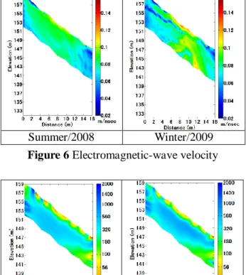
Figure 4 shows the P-wave velocity obtained by the seismic tomography method. This shows the tendency that the speed transmitted in the ground quickens as depth becomes deep. Figure 5 shows the S-wave velocity obtained by the surface wave method. A low-speed area is seen by about 4m in depth. Figure 6 shows the electromagnetic wave velocity obtained by the electromagnetic tomography method. It is shown the high percentage of water content if the electromagnetic velocity is slow, and the low percentage of water content if it is fast because the electromagnetic velocity depends on the water content in the ground.
Figure 7 shows the resistivity obtained by the resistivity tomography method. It is a low resistivity near the surface of the slope and it is a high resistivity in the middle depth.
Summer/2008 Winter/2009
Figure 4 P-wave velocity
Summer/2008 Winter/2009
Figure 5 S-wave velocity
A-district
B-district :Investigation line
Summer/2008 Winter/2009 Figure 6 Electromagnetic-wave velocity
Summer/2008 Winter/2009
Figure 7 Resistivity
(2) Self-organizing maps
Self-organizing maps is a kind of the neural net work developed by professor Kohonen of Helsinki university. This has the feature in which the input data of higher dimension data can be mapped to SOM plane of two dimensions in proportion to the degree of similarity. In a word, data with a different feature has the feature in which the map arranged at a position away can be made so that data with a similar feature is near. As a standard by which the degree of similarity is shown, Euclidean distance between data is used. It is judged that two data which this Euclidean distance is near looks like.
Moreover, SOM can cluster without the preliminary knowledge of data. The basis of the algorithm of SOM is shown in Figure 8.
First of all, the two-dimensional map is initialized. An individual neuron with the same dimension as the input vector is arranged in two dimension SOM plane at random besides the input vector.
Secondarily, it searches for the champion vector.
The champion vector is the one when Euclidean distance that shows the degree of similarity shown in the expression (1) is minimized. In a word, it looks for the most similar reference vector to the input vector.
21
n
k
jk ik j
i m x m
x
d (1)
Here, xi : the input vector, mj : the reference vector Thirdly, according to the expression (2) shown below, the champion vector and the circumference unit near the champion vector learn the input vector.
The neighborhood size is reduced as the learning progresses.
( ) ( )
) ( ) ( ) 1
(t m t h t x t m t
mi i ci i (2)
Here, mi(t) : information processing ability, hci(t) : the update rate, x(t) : the input vector.
The update rate is a ratio in which the champion vector and the vector near the champion vector is updated, and it is changed in proportion to the learn frequency as shown in expression (3).
2 ( )
) exp (
) ( )
( 2
2
t t t d
t hci
(3)
Here, α(t) : the learning coefficient, d(t) : the distance from the champion vector, σ(t) : the learning radius from the champion vector.
The learning coefficient and the learning radius from the champion vector are shown in the expression (4) and the expression (5). These
unspread the vector of the neuron by setting them to decrease with an increase in the learning frequency.
T
t) 1 t ( 0
(4)
T
t) 1 t ( 0
(5)
Here, α0 : the initial value of the learning coefficient, σ0 : the initial value of the learning radius, t : the learning frequency, T : All learning frequency
Fourthly, the SOM map is clustered. Repeating the search and the study of the vector a number of times, the vector with high similarity is arranged on the SOM map. And, considering those Euclidean distances makes it possible to classify the SOM map.
Finally, the input vectors classifies. By applying the input vectors to the clustering SOM map, it is understandable which class the input vectors are classified.
(1) Initialization of SOM map
(2) Search for champion vector
(3) Learning of champion vector and unit near it
(4) Clustering of SOM map
(5) Class separation of input vector Figure 8 The basis of the algorithm of SOM
(3) Adjustment of input geophysical data
As for the P-wave velocity, the S-wave velocity, the electromagnetic-wave velocity and the resistivity used by this research, the method of acquiring geophysical data is different. Therefore, the length of the investigation line, the exploration depth, and the sampling cell interval acquired are different. Then, we standardized the geophysical data interval with the interpolation of each geophysical data, and the cell interval, and unified the acquired geophysical exploration data as 0.5m.
The geophysical properties distributions acquired by each geophysical exploration shown from Figure 4 to Figure 7 have already been standardized. In addition, each geophysical data to input to SOM is different in the range of the maximum value and minimum value and the degree of variance value. Geophysical data that variance value is small reduces a relative influence on the output result by SOM. Therefore, we conducted a linear standardization to make the variance value one so that the importance of each data becomes equal.
(4) K-means method
In this paper, k-means method was used to classify objectively. K-means method sets the number of divided clusters first and classifies. On the characteristic of the calculation of k-means method, only the local optimum solution can be obtained, so a few differences are caused by the center position of an initial cluster in bottom-line.
Then, DB-index6) shown in the expression (6) as an evaluation function was used. An initial value of the number of patterns was set, and it was assumed that the result of minimizing DB-index was an appropriate classification. In this paper, to make a final classification result easy to interpret, the number of divided clusters was set to 4.
j i
j i
c
i i j X X
X X
DBindex c
max , 1
1
Here, c : Number of clusters, δ(Xi , Xj) : Euclidean distance between centers of cluster Xi and Xj, δ(Xi , Xj) : Euclidean distance between centers of cluster of cluster Xi and Xj
4. Classification of geophysical data by SOM with k-means method
The cluster distribution and the threshold of classification change if the SOM map of each data at each measurement time is made. Therefore, the data at all of the measurement time was brought together in one, the change of the cluster distribution and the threshold to classify was canceled. In this paper, the classification result by the data in Summer 2008 and Winter 2009 are shown as compound evaluations of measured geophysical data. Cluster boundary and distribution of physical value on the SOM map by k-means method are shown in Figure 9. The SOM map has no relation the vertical direction and the horizontal direction of two dimension plane, only arranges a similar vector in neighborhood. In Table 1, a relative amount of the geophysical value in each cluster is shown by the number of [●]. Comparisons of the classification result and the boring investigation are shown in Figure 10 and Figure 11.
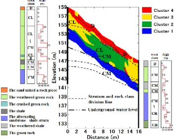
In the classification result in Summer 2008 in Figure 10 and Winter 2009 in Figure 11, the cluster 4 is corresponding to the area that RQD is 0%, the rock class is D-CL class, and the P-wave velocity and the resistivity is low, the Electromagnetic wave velocity is high in Table 1. Therefore, it is thought that the cluster 4 is the area that the moisture content is low, in other words, the permeability is
(6)
low and the weathering is progresses.The cluster 3 and the cluster 2 are corresponding to the area that RQD is 0-46%, the rock class is CL-CM class, the cluster 3 is that the P-wave velocity is middle, the S-wave velocity and the electromagnetic wave velocity is low, the resistivity is high in Table 1.
Therefore, it is thought that the cluster 3 is the area that the permeability is low though the crack of the rock progresses. The cluster 2 is that the P-wave velocity, the S-wave velocity and the resistivity are middle and the electromagnetic wave velocity is high in Table 1. Therefore, it is thought that the cluster 2 is the area that the crack of the rock less progresses than the cluster 3 and the permeability is high. The cluster 1 is corresponding to the area that RQD is 10-26%, the rock class is CM class, and the P-wave velocity and the S-wave velocity are high, and the electromagnetic wave velocity is middle and the resistivity is low in Table 1. Therefore, it is thought that the cluster 1 is the area that the permeability is relatively high and there is the bleeding channel or a saturated condition below the underground water level.
Table 1 The relative amount of the geophysical value in each cluster
Cluster Vp Vs Vel R
1 ●●● ●●● ●● ●
2 ●● ●● ●●● ●●
3 ●● ● ● ●●●
4 ● ●● ●●● ●
Figure 11 The comparison of the classification result in Winter 2009 and the boring investigation
Compared Figure 10 with Figure 11, distributions of the overall cluster are almost similar, however, some changes take place in the vicinity of the boundary of the cluster 2 and the cluster 3. It is thought as this cause that the moisture state in the vicinity of the boundary of the cluster 2 and the cluster 3 in the ground is (a) P-wave velocity (b) S-wave velocity
(c) Electromagnetic wave velocity
(d) Resistivity
(e) Cluster distribution on the SOM map by k-means method
Figure 9 Cluster boundary and distribution of physical value on the SOM map
Figure 10 The comparison of the classification result in Summer 2008 and the boring investigation
1 4 2
3
1 4 2
3
1
2 3 4
1 2 3 4
1
3 4 2
changeable. In a word, there is a possibility with the bleeding channel also in this vicinity.
5. CONCLUSION
In this research, the geophysical data was characterized and classified to 4 clusters by SOM with k-means method. The opinions obtained from this research are shown as follows.
1) By using 4 kinds of different dimensional geophysical value (the P-wave velocity, the S- wave velocity, the electromagnetic wave velocity, and the resistivity) that had been obtained from 4 kinds of geophysical explorations to classify SOM with k-means method, we got the result that is roughly corresponding to the degree of the rock class and RQD by the boring investigation
2) It can be said that this technique is effective for the improvement of the interpretative accuracy of two or more geophysical exploration evaluations because it can make it possible to read two or more geophysical exploration datum simultaneously and simply understand and evaluate the feature of each clusters on the SOM map. Therefore, it was shown to be able to do adjusted evaluation with the boring investigation by SOM with k-means method as the overall evaluation technique of two or more geophysical data.
3) It is thought that it is necessary to evaluate the change of the situation in the ground like the weathering and the aquifer situation.
ACKNOWLEDGMENT: When this research is advanced, I appreciate everybody of new urban society technology creation uniting study group
"Research about the engineered method of the slope ground by a continuous measurement of the geophysical exploration" project that offers the local measurement data.
REFERENCES
1) Kusumi, H., Nakamura, M. : Engineering Estimation Method of Rock Masses by Conversion Analysis Using Seismic Velocity and Electric Resistivity, 11th International Congress on Rock Mechanics (ISRM2007), pp861-864, 2007.
2) Kohonen,T.: Simulataneous order in nervous nets from a functional standpoint, Biological Cybernetics,Vol.50,pp.35-41,1982.
3) Kohonen, T.: Self-Organization and Associative Memory, Heidelberg: Springer,1984.
4) T.Tsuji, T.Matsuoka, K.Nakamura, E.Tokuyama, S. Kuramoto, Bangs Nathan L : Physical
properties along the plate boundary decollement in the Nankai Trough using seismic attributes analysis with Kohonen self-organizing map, Journal of Society of Exploration Geophysicists of Japan, Vol.57, No.2 (2004) pp.121-134.
5) A.Miyakawa, T.Tsuji, T.Matsuoka, T.Yamamoto: Self-organizing maps classification of soil properties in levee using different geophysical data, Journal of Japan Society of Civil Engineers C Vol. 66, No. 1, pp.89-99, (2010) .
6) Davies, D. L. and Bouldin, D. W.: A cluster separation measure, IEEE Transactions on Pattern Recognition and Machine Integrence, Vol.1, No.2, pp.224-227, 1979.