SUMMARY In this paper, we propose improved methods of liquid- phase detection of biological targets utilizing magnetic markers and a high-critical-temperature superconducting quantum interference device (SQUID). For liquid-phase detection, the bound and unbound (free) mark- ers are magnetically distinguished by using Brownian relaxation of free markers. Although a signal from the free markers is zero in an ideal case, it exists in a real sample on account of the aggregation and precipitation of free markers. This signal is called a blank signal, and it degrades the sensitivity of target detection. To solve this problem, we propose improved detection methods. First, we introduce a reaction field, Bre, during the binding reaction between the markers and targets. We additionally intro- duce a dispersion process after magnetization of the bound markers. Using these methods, we can obtain a strong signal from the bound markers with- out increasing the aggregation of the free markers. Next, we introduce a field-reversal method in the measurement procedure to differentiate the signal from the markers in suspension from that of the precipitated mark- ers. Using this procedure, we can eliminate the signal from the precipitated markers. Then, we detect biotin molecules by using these methods. In an experiment, the biotins were immobilized on the surfaces of large polymer beads with diameters of 3.3μm. They were detected with streptavidin- conjugated magnetic markers. The minimum detectable molecular number concentration was 1.8×10⁻¹⁹mol/ml, which indicates the high sensitivity of the proposed method.
key words: high-critical-temperature superconducting quantum interfer- ence device (SQUID), magnetic marker, immunoassays, liquid-phase de- tection
1. Introduction
Magnetic immunoassay techniques that utilize Brownian relaxation of magnetic markers have been developed for liquid-phase detection of biological targets[1]–[16]. In techniques of this type, the bound and free markers are magnetically distinguished using the Brownian relaxation of the markers. To date, several detection methods, including AC susceptibility[1]–[6], magnetic relaxation[7]–[13], and remanence measurement[14]–[16], have been developed.
These methods eliminate the need for a time-consuming washing process for marker separation.
We have therefore developed a liquid-phase detection technique that employs large polymer beads that immobi- lize the bound markers[14]–[16]. In this method, biological targets are fixed on the surface of large polymer beads with
Manuscript received October 23, 2015.
Manuscript revised December 24, 2015.
†The authors are with the Department of Electrical Engineer- ing, Kyushu University, Fukuoka-shi, 819–0395 Japan.
a) E-mail: [email protected] DOI: 10.1587/transele.E99.C.669
sizes typically on the order ofμm. In this case, the Brownian relaxation time of the bound marker becomes much longer than that of the free markers. Namely, the signal from the bound markers is retained for a long time period on account of the long relaxation times of the markers. On the other hand, the signal from the free markers rapidly decays to zero on account of their short relaxation times. As a result, the bound and free markers can be magnetically distinguished.
The signal from the free markers is zero in an ideal case; however, in a practical sample, the signal is present. In the practical sample, two types of markers exist in addition to the bound and free markers. One is the agglomerate of free markers. The other is comprised of the markers that are precipitated or absorbed on the bottom of the reaction well. Because the Brownian relaxation of these markers is deteriorated, the signal is generated from these markers[16].
This signal is called a blank signal, and it degrades the target detection performance. Therefore, it is necessary to solve this problem to further improve the detection sensitivity.
In this paper, we propose methods that can decrease the blank signal from the free markers. First, we present improved methods for sample preparation and magnetiza- tion of the bound markers. We introduce a reaction field, Bre=1.5 mT, during the binding reaction between the mark- ers and targets. We additionally introduce a dispersion pro- cess after magnetization of the bound markers. Next, we propose a measurement procedure to distinguish the signal from the markers in suspension from that of the precipitated markers. Using these methods, we can obtain a strong signal from the bound markers without increasing the blank signal of the free markers. Finally, we demonstrate the detection of biotin molecules. The minimum detectable molecular num- ber concentration is 1.8×10⁻¹⁹mol/ml, which indicates the high sensitivity of the proposed method.
2. Principle of Liquid-Phase Detection
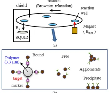
Figure 1 (a) schematically depicts the measurement system for liquid-phase target detection. As shown in Fig. 1 (b), bi- ological targets are fixed to large polymer beads with diame- ters ofdp=3.3μm. The magnetic markers are bound to the targets for detection. The bound and free markers coexist in the sample solution. The hydrodynamic diameter of the marker isdh =200 nm. The Brownian relaxation times of Copyright c2016 The Institute of Electronics, Information and Communication Engineers
(a)
(b)
Fig. 1 (a) Schematic diagram of the detection system, and (b) markers in the practical sample.
the free and bound markers are calculated using the relation τB=(πη/2kBT)d3, whereη=1×10⁻³Pa·s is the viscosity of water, kBis the Boltzmann constant,T =300 K, anddis the diameter of the particle. Using the values ofdh anddp ford, they are determined to beτB=6 ms and 13 s for the free and bound markers, respectively.
The sample solution, including both the bound and free markers, is placed in a reaction well, as shown in Fig. 1 (a).
The bound and free markers are magnetically distinguished by the difference between their Brownian relaxation times.
Details of this detection principle have been described else- where[16]. Briefly, a measurement field, Bmea = 1 mT, is applied to measure the magnetic (remanence) signals from the bound markers, as shown in Fig. 1 (a). When the sample plate is rotated and the reaction well is free from the mag- netic field of the magnet, so thatB = 0, the free markers undergo Brownian relaxation. AfterT =1.5 s, the reaction well is brought above the superconducting quantum interfer- ence device (SQUID). In that position, the signal from the free markers decays to zero; therefore, only the signal from the bound markers is detectable.
In our study, the signal from the markers is detected with a high-critical-temperature SQUID, which includes a ramp-edge Josephson junction[17]. The flux noise at 77 K is S1/2Φ = 7.5 μΦ0/Hz1/2 in the white noise region, and 14μΦ0/Hz1/2 at f = 1 Hz when SQUID is operated in the AC bias mode.
The sample plate has twelve reaction wells. By rotating the sample plate, we can measure the signal from each reac- tion well. Figure 2 depicts the waveform of the signals,Φ(t), which were obtained from the four reaction wells with dif- ferent concentrations of the targets (biotin molecules). As shown, the amplitude of the signal increases with the in- crease of the number of targets,NB. The peak-to-peak value of the signal is defined as the signal,Φs, from the markers
Fig. 2 Waveform of the signals from the four reaction wells with differ- ent concentrations of the targets (biotin molecules). The number of biotins isNB1=2×10⁴, NB2=5×10⁴, and NB3=105. The measurement field wasBmea=1 mT.
in each sample.
As shown in Fig. 2, the blank signal is obtained even in the absence of the target (i.e., for the case of NB = 0).
However, as noted above, it should be zero in the ideal case.
As depicted in Fig. 1 (b), the two types of markers—the ag- glomerate of free markers and those precipitated or absorbed on the bottom of the reaction well—exist in addition to the bound and free markers in the practical sample. As men- tioned, the Brownian relaxation of these markers is deterio- rated; accordingly, the blank signal is generated from these markers[16].
This blank signal affects the sensitivity of target detec- tion. To perform highly sensitive detection, the ratio be- tween the signal from the bound markers and the blank sig- nal must be increased. In the following section, we demon- strate the improvement in the detection procedure for this purpose.
3. Sample Preparation and Magnetization
In the experiment, we used biotin molecules as targets. Ap- proximately 1,300 biotins were conjugated to a single poly- mer bead. Streptavidin-conjugated magnetic markers (FG beads, Tamagawa Seiki) were put in the sample solution for detection. These markers were bound to the biotins, as illustrated in Fig. 1 (b). The binding reaction was per- formed for 60 min at 30◦C in a phosphate buffer solution.
For detection, 60 μL of the sample was deposited into a well, as shown in Fig. 1 (a). Concentration of the number of biotin-conjugated polymer beads was changed from 5 to 100/60μL in order to detect biotin molecules from 6.5×10³ to 1.3×10⁵/60μL. Concentration of the magnetic markers was 1μg/60μL. It should be noted that the N´eel relaxation time of the present marker is very long, and the marker gen- erates the remanence signal after magnetization[16].
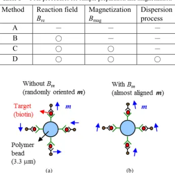
We studied four different methods for sample prepara- tion and magnetization, as listed on Table 1.
• In method A, the sample is prepared using a conven- tional technique.
(a) (b)
Fig. 3 Magnetic momentmof the bound markers at the end of the bind- ing reaction. (a)mis randomly oriented withoutBre. (b)mis almost aligned whenBreis applied.
• In method B, the sample is prepared using a reaction field,Bre=1.5 mT.
• In method C, the sample is magnetized after applying method B by using a magnetization field of Bmag = 40 mT.
• In method D, the dispersion process using a vortex stir- ring is performed after method C.
3.1 Binding Reaction Using Reaction FieldBre
First, we compared method A with method B, as listed in Table 1. Method A is a conventional sample preparation technique. Using method B, we introduced a weak mag- netic field during the binding reaction between the targets and markers. This field was denoted by the reaction field, Bre[18]. In Fig. 3, the effect of Bre is schematically pre- sented. In the absence ofBre, the markers rotate in the solu- tion during the binding reaction on account of the Brownian rotation. As a result, the magnetic moment,m, of the bound markers was randomly oriented when the binding reaction was finished, as shown in Fig. 3 (a). However, when field Bre was applied, the moments of the markers were aligned to the direction ofBreduring the reaction. Hence, the mark- ers were bound to the targets with their momentsmalmost aligned, as shown in Fig. 3 (b). This contrasted with the con- ventional case withoutBre. Owing to the alignment of the momentsm, the bound markers could be easily magnetized.
To determine the strength of field Bre, we measured the magnetization curve of the markers in the solution. In Fig. 4, the measured magnetic moment of the sample,<m>, is shown by circles when the weak field,H, is applied. It is well known that the value of the magnetic moment of the
Fig. 4 Low field magnetization curve of the markers in solution. Exper- imental value<m>can be divided into two terms,<m>=<m1>+<m2>.
marker,m, is distributed in the sample[19]. It is also shown that, for the markers that show remanence after magnetiza- tion, the distribution can be approximated by using two typ- ical values ofm[20]. Hence, we assume that<m>can be expressed by the sum of two terms,<m>=<m1>+<m2>.
Here, <m1> is given by the markers with small m val- ues, and it linearly increases with H. On the other hand,
<m2>is given by the markers with largemvalues, whose behaviors in solution are given by the Langevin function L(ξ)=coth(ξ)−1/ξwithξ=μ0Hm/kBT.
In Fig. 4, we show the<m1>-Hand<m2>-Hcurves.
<m1>is obtained from the linear part of the<m>-Hcurve at high values ofH, whereas<m2>is obtained by subtracting
<m1>from<m>. When we fit the<m2>-Hcurve with the Langevin function, we getm=2×10⁻¹⁷Am2.
As shown in Fig. 4,<m2>is saturated for the field val- ues greater than 1.5 mT. This means that markers with large mvalues are aligned in the solution by fieldH. Therefore, we selected reaction fieldBre=1.5 mT in the following ex- periment: We appliedBre = 1.5 mT for 60 min during the binding reaction between the targets and markers.
In Fig. 5 (a), the blank and bound signals obtained for methods A and B are shown. The blank signal indicates the signal from the free markers in the absence of targets, specifically when the number of biotin molecules isNB=0.
The bound signal indicates the signal from the markers that are bound to the targets whenNB=1.3×10⁵. By comparing the results of cases A and B, the effect of reaction fieldBre is evident.
As shown in Fig. 5 (a), the blank signal is almost the same for the A (Bre = 0) and B (Bre = 1.5 mT) cases.
This result reveals that the aggregation of the free markers due to reaction field Bre is very small. However, a larger bound signal is obtained for case B. The bound signal is in- creased by approximately five times compared to case A.
This is because the markers are bound to the targets with their momentsmalmost aligned when the reaction field of Bre=1.5 mT is used, as shown in Fig. 3 (b).
In Fig. 5 (b), the ratio between the bound and blank sig- nals defined by the following equation is shown.
(a)
(b)
Fig. 5 (a) Bound and blank signals obtained with four different methods.
Methods A to D are listed in Table 1. (b) Ratio between the bound and blank signals given in Eq. (1).
Ratio=Bound signal (NB=1.3×10⁵)
Blank signal (NB=0) (1) The ratios are 2.0 and 8.6 for cases A and B, respec- tively. Therefore, reaction fieldBreis useful for increasing the detection sensitivity.
3.2 Magnetization
As shown in Fig. 3 (b), magnetic momentsmof the bound markers were almost aligned when the reaction field was used. However, to completely alignm, additional magne- tization was required. We therefore applied magnetization fieldBmag.
In method C listed in Table 1, we applied the magne- tization field ofBmag =40 mT for 200 ms after the binding reaction was finished[16]. In Fig. 5 (a), the blank and bound signals obtained with this method are shown. By comparing the results with those of method B, the effect of magnetiza- tion fieldBmag is evident. As shown in Fig. 5 (a), both the blank and bound signals in case C increased compared to those of case B. The increase of the blank signal indicates that the magnetization fieldBmag caused agglomeration of the free markers. On the other hand, the increase of the bound signal indicates that the additional alignment ofmof the bound markers was caused byBmag.
In Fig. 5 (b), the ratio between the bound and blank sig- nals given by Eq. (1) is shown. In case C, the ratio is 6.0,
Fig. 6 Effect of the magnetization field on the blank and bound signals.
The magnetization process (Bmag=40 mT for 200 ms) was repeatedkmag
times with intervals of 3 s. The ratio between the bound and blank signals is given in Eq. (1).
which is smaller than the value of 8.6 obtained for case B.
This value is decreased because the rate of increase of the blank signal due to Bmag is larger than that of the bound signal.
To study the effect ofBmagon the blank and bound sig- nals, the magnetization process (Bmag=40 mT for 200 ms) was repeatedkmagtimes with intervals of 3 s. Note that we used kmag = 1 in the method C shown in Fig. 5. In Fig. 6, changes of the blank and bound signals are shown when kmagwas increased. Both signal types increased withkmag. On the other hand, the ratio given by Eq. (1) decreased with kmag. Therefore, the magnetization process decreased the detection sensitivity, although the bound signal increased.
Therefore, it is necessary to prevent the increase of the blank signal due toBmag.
3.3 Dispersion Process
To decrease the blank signal caused byBmag, we introduced a dispersion process afterBmag=40 mT was applied:kmag= 1 was used in the experiment. In method D listed in Table 1, the sample solution was vortex-stirred just after Bmag was turned off. If the binding force of the agglomerate, which was produced by Bmag, was weak, the agglomerate would be unraveled by the vortex stirring.
In Fig. 5 (a), the blank and bound signals obtained with method D are shown. By comparing the results with those of method C, the effect of vortex stirring is evident. As shown in Fig. 5 (a), the blank signal in case D decreased compared to case C. This result indicates that the agglomerate of the free markers was unraveled by the vortex stirring, as ex- pected. We note that the bound signal was also decreased by the vortex stirring. This result indicates that the aggre- gation between the bound and free markers was also caused by fieldBmagand that the agglomerate was unraveled by the vortex stirring.
In Fig. 5 (b), the ratio between the bound and blank signals given by Eq. (1) is shown. In method D, the ra- tio is 10.3. This value is the highest of the four methods.
Bmea = 1 mT. Then, the polarity of the measurement field was changed toBmea=−1 mT.
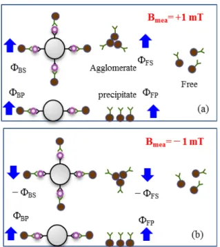
Figure 7 (a) shows the signals generated from the mark- ers when the field ofBmea =1 mT was used. There are four types of signals: ΦBS,ΦBP,ΦFS, andΦFPwere those from the bound markers in suspension, precipitated bound mark- ers, agglomerate of free markers in suspension, and precip- itated free markers, respectively. Therefore, the signal mea- sured in this case was given by
Φ(+)= ΦBS(NB)+BBP(NB)+ ΦFS+ ΦFP. (2) Note that signalsΦBSandΦBP, which were generated by bound markers, increased with the number of the targets, NB. On the other hand,ΦFSandΦFP, which were generated by free markers, were independent ofNB.
When the polarity of the measurement field was changed to Bmea = −1 mT, only the markers in suspen- sion could physically rotate with the magnetic force. There- fore, signalsΦBSandΦFSchanged the polarity, as shown in
Fig. 7 Signals from the markers in the practical sample after applying (a) Bmea= +1 mT, and (b) Bmes=−1mT. The four types of signals—ΦBS, ΦBP,ΦFS, andΦFP—were those from the bound markers in suspension, precipitated bound markers, agglomerate of free markers in suspension, and precipitated free markers, respectively.
and
Φ(+)+ Φ(−)
2 = ΦBP(NB)+ ΦFP. (5)
From Eq. (4), we can obtain the signals from the mark- ers in suspension. On the other hand, we can obtain the signals from the precipitated markers from Eq. (5). There- fore, we can differentiate the signals between the suspended and precipitated markers.
In Fig. 8, the experimental results are shown for the cases ofBmea = 1 mT and−1 mT. The samples were pre- pared by the method D mentioned in Sect. 3. The horizontal axis in Fig. 8 represents the number of biotin molecules,NB; the vertical axis represents the detected signal. The signal Φ(+) was obtained withBmea=1 mT, while the signalΦ(−) was obtained withBmea=−1 mT. As shown, the polarity of the signalΦ(−) was changed compared toΦ(+), as expected from Eqs. (2) and (3).
Using Eq. (4), we obtained the signalΦBS(NB)+ ΦFS
from the markers in suspension. The circles in Fig. 9 show the result. The signal increased with an increase inNB. This behavior indicates that the increase in the signalΦBS(NB) was generated by the bound markers. On the other hand, the signal atNB=0 representedΦFS. Note that signalΦFSwas generated by the agglomerate of free markers in suspension.
Using Eq. (5), we obtained the signalΦBP(NB)+ ΦFP
from the precipitated markers. The squares in Fig. 9 show the result. The signal was almost constant and independent
Fig. 8 Relationship between detected signalΦsand the number of biotin molecules,NB. SignalsΦ(+) andΦ(−) were obtained forBmea= +1 mT and−1 mT, respectively.
Fig. 9 Signal from suspended and precipitated markers. Signal ΦBS(NB)+ ΦFSwas obtained from Eq. (4) and represents the signal from markers in suspension. SignalΦBP(NB)+ ΦFPwas obtained from Eq. (5) and represents the signal from the precipitated markers.
ofNB. This result indicates thatΦBP(NB) was almost zero;
in other words, precipitated bound markers did not exist in this case. On the other hand, the signal atNB = 0 repre- sentedΦFP. This result means that precipitated free markers existed in this case. As shown in Fig. 9, the value ofΦFP
was nearly the same as that ofΦFSin the present case.
5. Detection Sensitivity
The relationship betweenΦBS(NB)+ ΦFSandNBshown in Fig. 9 was used to detect the biotin molecules. The mini- mum detectable number wasNB,min = 6,500. Considering that the sample volume was 60μL, this value corresponds to the molecular number concentration of 1.8×10⁻¹⁹mol/ml.
Since the typical sensitivity of the optical method called ELISA is around 5×10⁻¹⁸ mol/ml, this result indicated a high sensitivity of the present method.
6. Conclusion
In this paper, we presented improved methods for liquid- phase target detection. First, we presented a method for sample preparation and magnetization of bound markers.
We introduced a reaction field,Bre, during the binding re- action between the markers and targets. We additionally in- troduced a dispersion process after magnetization of bound markers. With these methods, we could obtain a strong sig- nal from the bound markers without increasing the blank signal of the free markers. Next, we presented a field- reversal measurement procedure that can differentiate the signal from the markers in suspension from that of the pre- cipitated markers. Finally, we demonstrated the detection of biotin molecules using the improved detection method. The minimum detectable molecular number concentration was 1.8×10⁻¹⁹ mol/ml, which indicates the high sensitivity of the present method.
Acknowledgments
This work was partly supported by Grant-in-Aid for Scien- tific Research (S) 15H05764, Japan Society for the Promo- tion of Science.
References
[1] J. Lange, R. K¨otitz, A. Haller, L. Trahms, W. Semmler, and W.
Weitschies, “Magnetorelaxometry—A new binding specific detec- tion method based on magnetic nanoparticles,” J. Magn. Magn.
Mater., vol.252, pp.381–383, 2002.
[2] H.L. Grossman, W.R. Myers, V.J. Vreeland, R. Bruehl, M.D. Alper, C.R. Bertozzi, and J. Clarke, “Detection of bacteria in suspension by using a superconducting quantum interference device,” PNAS U. S. A., vol.101, no.1, pp.129–134, 2004.
[3] D. Eberbeck, F. Wiekhorst, U. Steinhoff, K.O. Schwarz, A.
Kummrow, M. Kammel, J. Neukammer, and L. Trahms, “Specific binding of magnetic nanoparticle probes to platelets in whole blood detected by magnetorelaxometry,” J. Magn. Magn. Mater., vol.321, no.10, pp.1617–1620, 2009.
[4] F. ¨Oisj¨oen, J.F. Schneiderman, A.P. Astalan, A. Kalabukhov, C.
Johansson, and D. Winkler, “A new approach for bioassays based on frequency- and time-domain measurements of magnetic nanoparti- cles,” Biosens. Bioelectron., vol.25, no.5, pp.1008–1013, 2010.
[5] H.J. Hathaway, K.S. Butler, N.L. Adolphi, D.M. Lovato, R.
Belfon, D. Fegan, T.C. Monson, J.E. Trujillo, T.E. Tessier, H.C.
Bryant, D.L. Huber, R.S. Larson, and E.R. Flynn, “Detection of breast cancer cells using targeted magnetic nanoparticles and ultra- sensitive magnetic field sensors,” Breast Cancer Res., vol.13, R108, 2011.
[6] B.T. Dalslet, C.D. Damsgaard, M. Donolato, M. Strømme, M.
Str¨omberg, P. Svedlindh, and M. Hansen, “Bead magnetorelaxome- try with an on-chip magnetoresistive sensor,” Lab Chip, vol.11, no.2, pp.296–302, 2011.
[7] F. ¨Oisj¨oen, J.F. Schneiderman, M. Zaborowska, K. Shunmugavel, P. Magnelind, A. Kalaboukhov, K. Petersson, A.P. Astalan, C.
Johansson, and D. Winkler, “Fast and sensitive measurement of spe- cific antigen-antibody binding reactions with magnetic nanoparti- cles and HTS SQUID,” IEEE Trans. Appl. Supercond., vol.19, no.3, pp.848–852, 2009.
[8] K. Enpuku, Y. Tamai, T. Mitake, T. Yoshida, and M. Matsuo, “Ac susceptibility measurement of magnetic markers in suspension for liquid phase immunoassay,” J. Appl. Phys., vol.108, no.3, 034701, 2010.
[9] J.J. Chieh, S.-Y. Yang, H.-E. Horng, C.Y. Yu, C.L. Lee, H.L. Wu, C.-Y. Hong, and H.-C. Yang, “Immunomagnetic reduction assay using high-Tcsuperconducting-quantum-interference-device-based magnetosusceptometry,” J. Appl. Phys., vol.107, no.7, 074903, 2010.
[10] M.J. Chiu, H.E. Horng, J.J. Chien, S.H. Liao, C.H. Chen, B.Y.
Shih, C.C. Yang, C.L. Lee, T.F. Chen, S.Y. Yang, C.Y. Hong, and H.C. Yang, “Multi-channel SQUID-based ultra-high-sensitivity in- vitro detections for bio-markers of Alzheimer’s disease via immuno- magnetic reduction,” IEEE Trans. Appl. Supercond., vol.21, no.3, pp.477–480, 2011.
[11] R.S. Gaster, L. Xu, S.-J. Han, R.J. Wilson, D.A. Hall, S.J. Osterfeld, H. Yu, and S.X. Wang, “Quantification of protein interactions and solution transport using high-density GMR sensor arrays,” Nature Nanotech., vol.6, no.5, pp.314–320, 2011.
[12] A. Shoshi, J. Schotter, P. Schroeder, M. Milnera, P. Ertl, V.
Charwat, M. Purtscher, R. Heer, M. Eggeling, G. Reiss, and H.
Brueckl, “Magnetoresistive-based real-time cell phagocytosis mon- itoring,” Biosens. Bioelectron., vol.36, no.1, pp.116–122, 2012.
[13] X. Zhang, D.B. Reeves, I.M. Perreard, W.C. Kett, K.E. Griswold, B.
uid-phase detection of biological targets with magnetic markers and high Tc SQUID,” IEEE Trans. Appl. Supercond., vol.24, no.4, 1600105, 2014.
[17] A. Tsukamoto, S. Adachi, Y. Oshikubo, and K. Tanabe, “Design and fabrication of directly-coupled HTS-SQUID magnetometer with a multi-turn input coil,” IEEE Trans. Appl. Supercond., vol.23, no.3, 6353540, 2013.
[18] K. Enpuku, Y. Ueoka, T. Sakakibara, M. Ura, T. Yoshida, T.
Mizoguchi, and A. Kandori, “Liquid-phase immunoassay utilizing binding reactions between magnetic markers and targets in the pres- ence of a magnetic field,” Appl. Phys. Express, vol.7, no.9, 097001, 2014.
[19] T. Sasayama, T. Yoshida, M.M. Saari, and K. Enpuku, “Comparison of volume distribution of magnetic nanoparticles obtained from M-H curve with a mixture of log-normal distributions,” J. Appl. Phys., vol.117, no.17, 17D155, 2015.
[20] Y. Higuchi, S. Uchida, A.K. Bhuiya, T. Yoshida, and K. Enpuku,
“Characterization of magnetic markers for liquid-phase detection of biological targets,” IEEE Trans. Magn., vol.49, no.7, pp.3456–3459, 2013.
[21] A. Tsukamoto, T. Mizoguchi, A. Kandori, H. Kuma, N. Hamasaki, H. Kanzaki, N. Usuki, K. Yoshinaga, and K. Enpuku, “Development of a SQUID system using field reversal for rapidly detecting bacte- ria,” IEEE Trans. Appl. Supercond., vol.19, no.3, pp.853–856, 2009.
[22] M. Ura, Y. Ueoka, K. Nakamura, T. Sasayama, T. Yoshida, and K.
Enpuku, “New Detection Method of Biological Targets Based on HTS SQUID and Magnetic Marker,” IEEE ISEC 2015 proceeding (in press).
Masakazu Ura received the B. Eng. and M. Eng. degrees from Kyushu University in 2014 and 2016, respectively. During the mas- ter course in Kyushu University, he engaged in the development of SQUID system for biologi- cal immunoassay.
Kota Nakamura received the B. Eng. degrees from Kyushu University in 2015, and is now master course student of Graduate School of Informa- tion Science and Electrical Engineering, Kyushu University. He has been developing a high-sensitive detection method of biological targets based on highTcSQUID magnetometer.
Teruyoshi Sasayama received the B. Eng., M. Eng., and Dr. Eng. degrees from Kyoto Uni- versity in 2007, 2009, and 2012, respectively.
He is an Assistant Professor in the Faculty of Information Science and Electrical Engineer- ing, Kyushu University. He has been engaged in analysis of magnetic nanoparticle properties.
His current interest is the development of the al- gorithm for magnetic particle imaging.
Takashi Yoshida received the B. Eng., M.
Eng., and Dr. Eng. degrees from Kyushu Univer- sity in 1998, 2000 and 2003, respectively. He is an Associate Professor in the Faculty of In- formation Science and Electrical Engineering, Kyushu University. He has been engaged in the biomedical applications of magnetic nanoparti- cles. His current interest is the development of a magnetic particle imaging system.
Keiji Enpuku received the B. Eng., M. Eng., and Dr. Eng. degrees from Kyushu University in 1976, 1978 and 1981, respectively. He is a Pro- fessor in the Research Institute of Superconduc- tor Science and Systems, Kyushu University. He has been engaged in the superconducting elec- tronics. His current interest is the development of high performance highTc SQUID magne- tometer and its applications.