Good Group Sparsity Prior for Light Field Interpolation

(1)

Shu FUJITA^†a), Keita TAKAHASHI^†b),Members,andToshiaki FUJII^†^c),Fellow

SUMMARY A light field, which is equivalent to a dense set of multi- view images, has various applications such as depth estimation and 3D display. One of the essential problems in light field applications is light field interpolation, i.e., view interpolation. The interpolation accuracy is enhanced by exploiting an inherent property of a light field. One example is that an epipolar plane image (EPI), which is a 2D subset of the 4D light field, consists of many lines, and these lines have almost the same slope in a local region. This structure induces a sparse representation in the frequency domain, where most of the energy resides on a line passing through the origin. On the basis of this observation, we propose a group sparsity prior suitable for light fields to exploit their line structure fully for interpolation. Specifically, we designed the directional groups in the discrete Fourier transform (DFT) domain so that the groups can represent the concentration of the energy, and we thereby formulated an LF interpolation problem as an overlapping group lasso. We also introduce several techniques to improve the interpolation accuracy such as applying a window function, determining group weights, expanding processing blocks, and merging blocks. Our experimental results show that the proposed method can achieve better or comparable quality as compared to state-of-the-art LF interpolation methods such as convolutional neural network (CNN)-based methods.

key words: light field reconstruction, group sparsity, discrete Fourier transform, epipolar plane image, line structure

1. Introduction

A light field (LF)[1],[2], which is equivalent to a set of multi-view images, is a useful data representation for both computer vision and graphics applications such as depth estimation[3],[4], digital refocusing[5],[6], and 3D displays[7],[8]. 3D visual information can be represented as a 4D LF signal with spatial(u, v)and angular(s,t)coordi- nates at/with which light rays pass a reference plane. Thus, to capture the LF signals, we can use camera arrays[9]and lenslet cameras[5],[10]. However, they have issues in terms of hardware such as extensive setting costs and a trade-off between the spatial and angular resolutions. As a result, the resolution of the captured LFs has a limit.

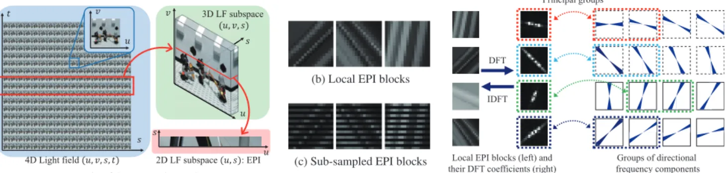
One of the solutions for this issue is LF interpolation[11]–[17], which is obtaining sufficiently dense views from the sparser views. As an example, Fig. 1(a) shows a 4D LF on(u, v,s,t)and its subspace. A section of the original LF with a fixed(v,t)is called an epipolar plane image (EPI).

Manuscript received November 5, 2018.

Manuscript revised August 24, 2019.

†The authors are with Graduate School of Engineering, Nagoya University, Nagoya-shi, 464-8603 Japan.

a) E-mail: [email protected] b) E-mail: [email protected] c) E-mail: [email protected]

DOI: 10.1587/transfun.2018EAP1175

As shown in Fig. 1(b), EPIs consist of many slanted lines that have almost the same slope in a local region. The line structure is one of the inherent properties of EPIs. Inter- polation of an LF, i.e., view interpolation, can be regarded as the problem of reconstructing the latent EPIs (Fig. 1(b)) from sparsely sampled EPIs shown in Fig. 1(c). In doing so, exploiting the line structure of an LF would help predict the missing samples. Technically speaking, the line structure induces a sparse representation in the frequency domain, where most of the energy concentrates on a line passing through the origin[18], as shown on the left of Fig. 1(d). The line of energy concentration in the frequency domain is orthog- onal to the dominant slanted angle in the corresponding EPI block.

On the basis of this observation, we propose a novel prior suitable for LFs, agroup sparsity prior, to exploit their line structure fully for LF interpolation. We focus on the energy concentration in the frequency domain like the ones shown on the left of Fig. 1(d). This energy concentration can be represented with a group sparsity if we define a set of directional groups in the frequency domain as shown on the right of Fig. 1(d). This sparsity model is applied to small EPI blocks, because they often have almost constant slopes, resulting in good energy concentration in the frequency domain, and discrete Fourier transform (DFT) is adopted for the frequency representation. However, the DFT-based reconstruction often suffers from windowing effects, which degrade the interpolation accuracy. Hence, we also introduce several implementation techniques to mitigate the effects and to increase the accuracy: block expansion, a window function, group weights, and block merging. Our experimental results show that our method has good interpolation accuracy and is comparable or superior to the state-of-the-art convolutional neural network (CNN)-based method[17].

The preliminary discussion of our group sparsity prior has been presented in[19]. In the present paper, we improved the interpolation accuracy by introducing several additional implementation techniques. Moreover, we exhaustively eval- uated the performance of our method.

The remainder of this paper is organized as follows.

Section 2 describes the background of our method including the related LF interpolation methods and a signal reconstruction framework using sparsity and group sparsity. In Sect. 3, we apply this framework to the problem of LF interpolation and derive a group sparsity prior that is suitable for LFs.

The proposed prior is experimentally validated in Sect. 4, followed by the conclusion in Sect. 5.

(2)

Fig. 1 Light field structure and concept of our group sparsity prior. DFT and IDFT mean discrete Fourier transform and inverse DFT. In the DFT domain, most of the energy of the line structured signals concentrates on a few directional groups.

2. Background

2.1 Light Field Interpolation

The trade-off between the spatial and angular resolutions is an essential issue in capturing LFs. To tackle this issue, several methods have been studied to increase the spatial and angular resolutions[4],[20],[21]. In this paper, we particularly focus on the view interpolation methods to increase the angular resolution.

The major approach to interpolate the views is to estimate depth maps and then to synthesize new views based on the estimated depth. Fortunately, state-of-the-art methods [3], [4], [22]–[25] have been developed to estimate the accurate depth maps. However, these depth-based ap- proaches[3],[4],[22]–[25]suffer from artifacts, e.g., ghosting and tearing effects, in occluded and textureless regions.

Kalantari et al.[16]proposed a learning-based reconstruction method using two sequential CNNs to further increase the interpolation accuracy. The two CNNs were designed for depth estimation and view synthesis, respectively, and they were simultaneously trained so that the errors between synthesized and ground truth images are minimized. As a result, the CNN-based method achieved high-quality view interpolation for real scenes.

Another approach uses prior knowledge of LFs effec- tively to interpolate the views directly. One of the represen- tatives is a prior described in the frequency domain. Levin and Durand[11]assumed a Lambertian model and utilized Gaussian priors based on the dimensionality gap [6] that 4D LFs are essentially bounded within a 3D subspace in the frequency domain. Shi et al.[13]focused on the fact that LFs are extremely sparse in the continuous Fourier domain and used them to interpolate LFs. Vagharshakyan et al.[14]and Sahin et al.[15]found that EPIs become sparse in the shearlet domain[26], and they formulated LF interpolation as sparse coding. In addition, several priors other than frequency-domain based ones are also discussed. Mi- tra and Veeraraghavan[21]introduced a Gaussian mixture model (GMM) prior based on roughly estimated disparities

to model LF patches. Heber and Pock[27]formulated a prior that EPIs become low-rank when they are sheared adaptively according to their slopes.

Recently, Wu et al.[17]have proposed a CNN-based method on the EPI domain, which achieves the best interpolation quality among the recent interpolation methods.

Although this CNN-based method is successful in produc- ing high-quality results, it lacks scalability, i.e., the CNNs should be retrained for each condition; if the scaling factor is changed, the networks should be retrained.

2.2 Sparsity and Group Sparsity

Here, we describe a reconstruction framework ofa general signalusing sparsity and group sparsity, which is well known as sparse coding. An extension to the case of LF signals is discussed in 3.

Let x ∈ R^N be a target signal, and let y ∈ R^N be the observation from whichxshould be reconstructed. The observation model is given by

y=Φx, (1)

whereΦ ∈R^N^×N is an observation matrix, which depends on the types of reconstruction such as super-resolution and denoising. We assume that x is represented using a linear combination ofMcolumn vectorsa1, . . . ,aM ∈R^Nand the coefficientsz₁, . . . ,z_M, and that it is written as

x=Az, (2)

wherez =(z₁, . . . ,z_M)^T is the coefficient vector, and A= (a1, . . . ,aM)is generally called a basis or frame.

A key assumption in sparse coding is that vector z should be sparse; only a few elements take non-zero values.

With convex relaxation of this sparsity prior, a sparse vector ˆ

zcan be derived by solving a lasso problem[28]as follows.

ˆ

z=arg min

z

||y−ΦAz||²₂+λ||z||₁¹, (3) whereλis a non-negative parameter, and wherek·k₁andk·k₂ arel1andl2 norms, respectively. For further introducing a

(3)

||z||_G= X

gi∈ G

w_i||zgi||¹

2, (5)

whereηis a non-negative parameter. Vectorzgiincludes all the elements ofzthat belong to thei-th group. The set ofg_i is described asG={g₁, . . . ,g| G |}, where|G |is the number of groups. Symbolw_iis the weight for thei-th group. This problem written as Eq. (4) is called a sparse group lasso[29]

or an overlapping group lasso[30],[31]depending on the existence of overlapped coefficients between groups.

3. Group Sparsity Prior

In this section, we propose a group sparsity prior suitable for light fields to fully exploit their line structure for the problem of LF interpolation. Furthermore, we also introduce several implementation techniques to increase the interpolation accuracy: block expansion, a window function, group weights, and block merging.

3.1 Basic Formulation 3.1.1 Notation

We apply the aforementioned sparsity and group sparsity to the LF interpolation problem by interpreting the notations used in Sect. 2.2 as follows. Vectorsx andyare latent and observed LF signals. In this paper, the processing unit for the LF is a 2D block extracted from a 2D EPI; therefore, it is reshaped from 2D to 1D to yield a vector representation used asxory. The observation matrixΦis a sub-sampling operator in the angular domain in the case of view interpolation, but it can be adapted to other applications. For example,Φ is an identity matrix in the case of denoising and is a spatial down-sampling operator in the case of spatial super-resolution. In other words, we can process various reconstructions by controlling the observation matrix.

The design ofAis important because it determines the domain where the sparsity and group sparsity are consid- ered. A learned dictionary[24],[32], weighted discrete co- sine transform basis[33], and shearlet frame[14],[15]have been used for sparse representations of LFs. Meanwhile, we use the discrete Fourier transform (DFT) basis because it enables us to represent the line structure of an LF signal sparsely, as shown in Fig. 1. Note that the DFT coefficients are complex. In this paper, we simply replace kzk¹

1 with kRe(z)k¹

1+kIm(z)k¹

1, where Re(z)and Im(z)are the real and imaginary parts, respectively. Another possible implementation (which is not adopted in this paper due to the complex- ity) is to replace|z|₁¹ withPM

k=1

q

kRe(z_k)k₁²+kI m(z_k)k²

1, whereRe(z_k)andI m(z_k)are grouped together to impose a joint sparsity constraint on the real and imaginary parts of

As shown in Fig. 1, the line structure in the spatial domain leads to sparse coefficients in the DFT domain. More- over, these coefficients mostly concentrate on a line passing through the origin, and the direction of which is perpendic- ular to that of the lines in the spatial domain. On the basis of this observation, we designed the group and group weights that are suitable for representing EPIs.

Figure 1(d) illustrates the basic concept of our group design, where the DFT coefficients are divided into a set of groups in accordance with the directions. The aforementioned observation reveals that the non-zero DFT coefficients will exist in only a few groups. In other words, the DFT coefficients will be group sparse over the aforementioned set of groups. This concept is practically implemented as follows. First, the lower frequency components are gathered in a group regardless of the directions because these components are likely to exist in any EPI. These frequency components are assigned to the first group g₁, and only the remaining coefficients are assigned to other groupsg_i (i=2, . . . ,|G |).

Second, we only consider the upper hemisphere in the frequency domain because the DFT coefficients that are sym- metric with respect to the origin are complex conjugate.

Therefore, the angle between 0 andπis equally divided into the |G | −1 sub-angles, and the principal direction of the groupg_iis determined by

θ_i= (i−2)π

|G | −1, i=2, . . . ,|G |. (6) Finally, we allow the coefficients to overlap between the adjacent groups because the coefficients are defined over only the discrete set of frequencies, while the direction is continuous in nature. Basically, each of the DFT coefficients is assigned to the group that is nearest in terms of the direction.

However, the DFT coefficients that saddle on two adjacent directions are assigned to both of the groups. An example of the groups is shown in Fig. 2. Here, the dotted black lines indicate the approximate boundaries for the directional groups, where the discrete DFT coefficients are assigned to the groups approximately in accordance with Eq. (6).

Fig. 2 Example of group design in DFT domain.

(4)

3.2 Implementation

Our method consists of block-wise operations because it is designed for relatively small processing units (2D EPI blocks), e.g., 17×17 and 9×9 pixels. These EPI blocks are extracted from the input LFY, interpolated using our DFT-based group sparsity prior, and are written back to the corresponding position of the output LF X. However, the block-wise operation causes annoying window effects, which disturb the sparseness and group structure in the frequency domain. Furthermore, sub-sampled EPIs blocks like the ones shown in Fig. 1(c) are subject to aliasing effects in the frequency domain, and these effects also disturb the frequency structure of EPIs. Thus, we introduce four implementation techniques to increase the interpolation quality:

expanding EPI blocks, applying a window function to the EPI blocks, determining group weights, and merging blocks into the complete EPI considering the window functions.

3.2.1 Expanding EPI Blocks

The interpolated signal tends to be distorted if both ends of the signal take different values because DFT assumes the periodicity for the input signal. It causes severe ghosting effects, especially in blocks having step edges. To suppress these effects, we expand the block by one pixel in both the spatial and angular directions. When the expanded pixels around the original block have no information in the original LF Y, the pixel values are set to 0. We also expand the observation matrix, setting 0 to the entries that correspond to the extended pixels. After interpolation using the expanded blocks, we retain only the pixels that are included in the original block.

3.2.2 Applying a Window Function

To suppress the negative effects caused by the window effects, we also apply a window function to the observed EPI signalyafter the mean µof the non-zero elements ofyis subtracted:

y⁰=W(y−µ), (7)

whereW ∈R^N^×N is a diagonal matrix encoding the Kaiser window function, the tails of which are set to non-zero values to make W invertible^†. Instead of y itself, y⁰ is used as the observation signal for reconstruction, from which the optimal ˆz is derived. Consequently, the interpolated LF is obtained as:

ˆ

x=W⁻¹Azˆ+µ. (8)

†We can use zero-tails window functions as well if we care for the division by zero in Eq. (8). In this case, the boundary pixels are finally nullified in Eq. (15).

3.2.3 Determining Group Weights

The sub-sampled EPI signal y⁰often contains aliasing artifacts due to the reduced sampling rate on the angular domain.

The aliasing effects produce DFT coefficients on different directions from those of the sufficiently sampled EPI signal.

The group weightsw_iin Eq. (5) should be determined to nul- lify the coefficients caused by aliasing effects. We compute w_i using the difference between the direction of each group θ_iand a pre-estimated direction for the latent EPI ˆθ:

w_i =sin(|θˆ−θ_i|) i=2, . . . ,|G |, (9) where 0 ≤ θ, θˆ _i < π. We experimentally determined w₁ =min(w_i) (i =2, . . . ,|G |). The pre-estimated direction for the latent EPI ˆθis computed from the sub-sampled EPI signaly⁰given as the input. The derivation details of ˆθ are mentioned in the following.

An EPI block is originally defined over the 2D space as fk,l with the discrete spatial coordinate(k,l)(0 ≤k,l <

√

N). The DFT coefficient of f_k,lis denoted asF_m,n, where

−b

√ N

2 c ≤m,n≤ b

√ N

2 c. The purpose is to find a line equa- tionn=mtanθin the DFT domain that fits the distribution of F_m,n. Specifically, we solve the weighted least square problem given as

θˆ=arg min

θ

X

m,n

Ψ_m,n||n−mtanθ||²₂. (10) The weight termΨ_m,nis designed as

Ψ_m,n =|Fm,n|²h²_m,nbm,n. (11) The first term is the energy of the coefficientF_m,n obtained from the observed EPI y⁰. The second term reduces the weight for higher frequency components to suppress the effect of aliasing that is caused by the sparse sampling of the EPI. In this paper, we utilize the Hann window function for the second term defined as

h_m,n=1−cos 2π^m+^bR/2_R ^b 2

1−cos 2πⁿ⁺^bR/2b_R 2

, (12) whereRis the window length, which depends on the ratio of sub-sampling because the aliasing effect happens beyond the Nyquist frequency. For example, if square EPI blocks are sub-sampled by a factor of 2 in the angular domain, we set R = d

√ N

2 e. Exceptionally, the second term is set to 0 when |m|,|n| > R. The third term is the weight for robust estimation[34], which is iteratively updated using the previous estimation of ˆθas

b_m,n=







1− dm,n/κ22

|dm,n| ≤κ

0 otherwise (13)

d_m,n= |n−mtan ˆθ|

p1²+tan²θˆ, (14)

(5)

Fig. 3 Estimating direction in frequency domain. In this figure, the target application is angular super-resolution. The left-top DFT coefficients are computed from a sub-sampled EPI block with black stripes.

whereκis a positive constant. Here, Eq. (14) computes the distance between the point(m,n) and the line, andb_m,nis initially set to 1.

The overview of direction estimation is shown in Fig. 3.

The estimated direction ˆθ is used to determine the group weights in accordance with Eq. (9).

3.2.4 Merging Blocks into a Complete EPI

In the final step of interpolation of an LF, each interpolated EPI blockxis written back to the corresponding position of the target LFX. Here, interpolated EPI blocks are denoted again asx_k(s,u)(k=1, . . . ,K), whereKis the number of total blocks. We assume that the interpolated EPI blocks x_k(s,u)are initially made to overlap each other. In our case, adjacent EPI blocks overlap by the half size of the block (rounded up after a decimal point) each other. Therefore, the overlapped EPI blocks are merged using weighted averages:

• Compute meansµfromy

• Compute input EPI blocks:y⁰=W(y−µ) Main processes:

• Determine group weightwfromy⁰(Eq. (9))

• Compute optimal coefficient by solving Eq. (4):

ˆ

z←overlappingGroupLasso(y⁰,ΦA, λ, η,G,w) Post-process:

• Reconstruct the EPI block ˆx←W⁻¹Azˆ+µ Reconstruct LF signalXfrom EPI blocks ˆx(Eq. (15)) Output:interpolated LF signalX

Xv,t(s,u)=

Pk∈Bv,t(s,u)Wk(s,u)x_k(s,u) P

k∈Bv,t(s,u)W_k(s,u) , (15)

where X_v,t(s,u)is an EPI of the target LF X with a fixed (v,t), and whereB_v,t(s,u)contains all the indices of the interpolated EPI blocks that include the pixel(s,t,u, v). Here, W_k(s,u)is the weight that the pixel(s,u)received from the window functionW ink-th blockx_k(s,u).

3.3 Overview of Our Method

To conclude, the entire procedure of our method is described in Alg. 1. Because our method consists of block-wise operations, we first extract EPI blocksyfrom the observed LFY and expand them. After applying the window function to the blocks, they are interpolated using our group sparsity prior.

Finally, the interpolated EPI blocksxare written back to the corresponding positions of the target LF X. These blocks are made to overlap each other, so the interpolation results are merged according to the weights given by the window function.

4. Experimental Results

We tested the performance of our group sparsity prior using Stanford LF datasets[35], new HCI LF datasets[36], and Wang et al.’s dataset [37]as the input LFs. Each dataset has 17×17, 9×9, and 7×7 views, respectively. Thus, the processing units were 17×17, 9×9, and 7×7 EPI 2D blocks, and these blocks are further expanded as mentioned in Sect. 3.2.1, i.e., √

N = 19, 11, or 9. We demonstrated view interpolation from the sub-sampled LFs, the views of which were alternatively sampled from the original LFs.

When handling a 2-D (s,t) viewpoint arrangement, we first performed interpolation insdirection and then intdirection sequentially

To implement our method, we divided the DFT coefficients into log₂√

N +1 groups, where g₁ is allocated to the 7×7, 5×5, and 3×3 low frequency components around the DC component for 17×17, 9×9, and 7×7 block sizes, respectively, and the remaining groups are assigned to directional high frequency components. To solve

(6)

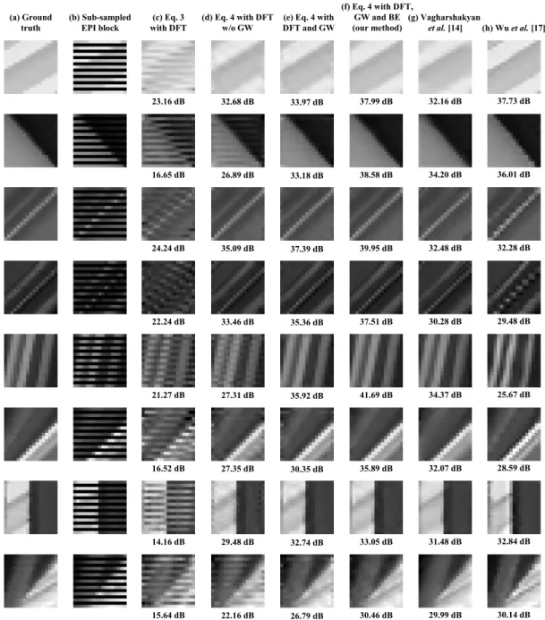
Fig. 4 View interpolation in the EPI domain. GW and BE represent group weight and block expansion, respectively.

Table 1 PSNR [dB] of the entire LFs after interpolating 9×9 views from 5×5 views.

Dataset[36] bedroom bicycle boxes cotton dino dishes greek herbs kitchen pillows tower Average Vagharshakyan et al.[14] 30.03 26.38 30.42 37.67 32.17 26.17 30.91 28.62 27.58 29.70 29.55 29.93 Kalantari et al.[16] 30.57 26.24 29.97 38.72 30.94 23.84 27.21 26.43 28.52 29.19 26.35 28.91

Wu et al.[17] 34.39 31.32 34.29 42.51 37.62 26.52 32.35 29.97 33.22 30.85 30.73 33.07

Eq. (3) with DFT 29.65 25.57 28.56 35.41 30.39 25.69 28.55 27.67 27.11 28.61 28.33 28.68

Eq. (4) with DFT w/o GW 34.20 30.91 34.80 40.53 36.27 28.45 33.27 30.66 32.15 32.75 30.93 33.18 Eq. (4) with DFT and GW 36.83 34.21 37.52 43.62 40.27 30.02 34.61 32.15 36.51 35.25 32.19 35.74 Eq. (4) with DFT, GW, and

BE (Our method)

38.72 36.34 39.63 45.69 42.87 30.89 35.74 33.12 38.91 37.70 32.83 37.49

Eq. (4), we used the SLEP library[38]. We compared our method with three state-of-the-art LF interpolation methods:

the Vagharshakyan et al.’s method[14], the Kalantari et al.’s

method[16], and the Wu et al.’s method[17]. The Vaghar- shakyan et al. method is a sparse coding method (Eq. (3)) using the shearlet frame [26] for interpolating EPIs. The

(7)

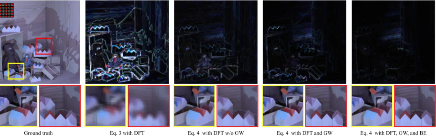
Fig. 5 Differences between ground truth and interpolated images (magnified by 5) at the (2, 2) viewpoint, which is among the 9×9 views interpolated from 5×5 views.

Fig. 6 Differences between ground truth and interpolated images (magnified by 5) at the (2, 2) viewpoint, which is among the 9×9 views interpolated from 5×5 views.

Fig. 7 PSNR of each view in a horizontal line in “dino”[36]. We enabled all the options except for BE.

Kalantari et al.’s method is based on explicit depth estimation followed by view interpolation using CNNs. The Wu et al.’s method is also a CNN-based method, but it does not need explicit depth estimation but interpolates views using a CNN on the EPI domain. We implemented the Vagharshakyan et al.

method using the MATLAB code with ShearLab[39],[40].

For this implementation, we found that using the pre/post- processings of Eqs. (7) and (8) improves the accuracy of the

Vagharshakyan et al.’s method[14]. Therefore, we also applied these processings to this method. For the Kalantari et al.’s method[16], and the Wu et al.’s method[17], we used each author’s distributed MATLAB codes. In all our experi- ments, we sought the best parameters for these methods and used them.

Figure 4 shows the results of view interpolation for several 17×17 EPI blocks. The ground truth and sub-sampled EPI blocks are shown in Figs. 4(a) and (b). Figures 4(c)–(f) are presented to show the contributions of the group sparsity, group weights (GW), and block expansion (BE) to the interpolation accuracy of our method. Our method can well interpolate EPI blocks even if they have multiple and con- tinuously varying slopes (see the two EPI blocks from the bottom). Figures 4(g) and (h) show the results of the Vaghar- shakyan et al.’s method[14]and Wu et al.’s method, which are inferior to those of our method.

Figures 5 and 6 show the difference of resulting images and ground truth at the same viewpoint that was missing in the input LFs but was interpolated by our method, the Vagharshakyan et al.’s method [14], Kalantari et al.’s method[16], and the Wu et al.’s method[17]. We can see that the group sparsity and group weights can suppress blur- ring and artifacts. The BE technique also contributed to

(8)

Fig. 8 Interpolated images at the (2, 2) viewpoint, which is among the 7×7 views interpolated from 3×3 views.

Table 2 PSNR [dB] of the entire LFs after interpolating 7×7 views from 3×3 views in Wang et al.’s dataset[37].

Average over 21 LFs Kalantari et al.[16] 32.62

Wu et al.[17] 37.27

Our method 37.02

suppressing the ghosting effect. The improvement brought by the BE technique is particularly large for the viewpoints near the outermost views (view number 1, 2, 8, 9) as shown in Fig. 7, which shows the accuracy of each view on a horizontal line. Moreover, we confirm that our method has less errors than the state-of-the-art methods.

Table 1 summarizes the performance comparison over ten datasets included in the new HCI LF dataset[36]. In the table, we also show the results of the other state-of-the-art methods of view interpolation[14],[16],[17]. We found that our method is superior to the other state-of-the-art methods.

Table 2 also summarizes the performance comparison for 21 LFs included in the Wang et al.’s dataset[37]. While the dataset[36]mentioned in Table 1 consists of computer generated scenes without noise, the dataset[37]mentioned Table 2 includes real scene captured by Lytro Illum cameras.

For this reason, the ground truth in this dataset includes noise, and thus, the PSNR values reported in Table 2 are only for reference. We can see that our method achieves comparable performance to the Wu et al.’s method, and the visual difference is imperceptible as shown in Fig. 8.

Finally, we mention the processing time. We executed

our method and the competitors on MATLAB R2019a with a 3.60 GHz Intel Core i9-9900K CPU without GPU acceler- ation. For view interpolation of an entire dataset, where 9×9 views were generated from 5×5 views in 512×512 pixels, our method took 1093 sec. Meanwhile, Vagharshakyan et al.[14], Kalantari et al.[16], and the Wu et al. [17]took 7716, 1628, and 1647 sec, respectively.

5. Discussion and Conclusion

5.1 Discussion

Our group sparsity prior described in the DFT domain was proposed for LF interpolation. However, it is formulated based on a general sparse coding framework, and thus, it has the possibility of being applied to not only LF interpolation but also the other applications that can be defined with an observation matrix. This flexibility to various applications is a benefit for our prior. It is hard to achieve such flexibility using CNN-based methods. Moreover, our prior in the DFT domain would be useful to design a better CNN- based method for LF processing because domain-specific knowledge has been shown to be effective in constructing CNNs[16],[17],[41].

5.2 Conclusion

Aiming to achieve light field interpolation with high-quality, we proposed a group sparsity prior in the discrete Fourier

(9)

processing blocks, applying a window function, determining group weights, and merging blocks.

Our experimental results show that our method achieved better quality than other state-of-the-art methods[14],[16]

and that it is superior or comparable to the latest convolutional neural network (CNN)-based method[17]. In future work, our group sparsity prior will be extended to the full 4D DFT domain of the light field to better utilize their structure. We will also investigate how the prior knowledge in the DFT domain can be used for designing better CNN-based methods for light fields.

References

[1] M. Levoy and P. Hanrahan, “Light field rendering,” ACM SIG- GRAPH, pp.31–42, 1996.

[2] S.J. Gortler, R. Grzeszczuk, R. Szeliski, and M.F. Cohen, “The lumigraph,” ACM SIGGRAPH, pp.43–54, 1996.

[3] M.W. Tao, S. Hadap, J. Malik, and R. Ramamoorthi, “Depth from combining defocus and correspondence using light-field cameras,” IEEE International Conference on Computer Vision (ICCV), pp.673–680, 2013.

[4] S. Wanner and B. Goldluecke, “Variational light field analysis for disparity estimation and super-resolution,” IEEE Trans. Pattern Anal.

Mach. Intell., vol.36, no.3, pp.606–619, 2014.

[5] R. Ng, M. Levoy, M. Bredif, G. Duval, M. Horowitz, and P. Han- rahan, “Light field photography with a handheld plenoptic camera,”

Stanford University Computer Science Tech Report CSTR, 2005.

[6] R. Ng, “Fourier slice photography,” ACM Trans. Graph., vol.24, no.3, pp.735–744, 2005.

[7] G. Wetzstein, D. Lanman, M. Hirsch, and R. Raskar, “Tensor displays: Compressive light field synthesis using multilayer displays with directional backlighting,” ACM Trans. Graph., vol.31, no.4, pp.1–11, 2012.

[8] K. Takahashi, Y. Kobayashi, and T. Fujii, “Displaying real world light fields using stacked LCDs,” International Display Workshops in conjunction with Asia Display, pp.1300–1303, 2016.

[9] B. Wilburn, N. Joshi, V. Vaish, E.V. Talvala, E. Antunez, A. Barth, A. Adams, M. Horowitz, and M. Levoy, “High performance imag- ing using large camera arrays,” ACM Trans. Graph., vol.24, no.3, pp.765–776, 2005.

[10] A. Lumsdaine and T. Georgiev, “The focused plenoptic camera,” IEEE International Conference on Computational Photography (ICCP), pp.1–8, 2009.

[11] A. Levin and F. Durand, “Linear view synthesis using a dimensionality gap light field prior,” IEEE Conference on Computer Vision and Pattern Recognition (CVPR), pp.1831–1838, 2010.

[12] S. Wanner and B. Goldluecke, “Spatial and angular variational super- resolution of 4D light fields,” European Conference on Computer Vision (ECCV), pp.608–621, 2012.

[13] L. Shi, H. Hassanieh, A. Davis, D. Katabi, and F. Durand, “Light field reconstruction using sparsity in the continuous Fourier domain,”

ACM Trans. Graph., vol.34, no.1, pp.12:1–12:13, 2014.

[14] S. Vagharshakyan, R. Bregovic, and A. Gotchev, “Image based rendering technique via sparse representation in shearlet domain,” IEEE International Conference on Image Processing (ICIP), pp.1379–

1383, 2015.

[15] E. Sahin, S. Vagharshakyan, J. Mäkinen, R. Bregovic, and A. Gotchev, “Shearlet-domain light field reconstruction for holo- graphic stereogram generation,” IEEE International Conference on

field reconstruction using deep convolutional network on EPI,” IEEE Conference on Computer Vision and Pattern Recognition (CVPR), 2017.

[18] J.X. Chai, X. Tong, S.C. Chan, and H.Y. Shum, “Plenoptic sampling,”

ACM SIGGRAPH, pp.307–318, 2000.

[19] K. Takahashi, S. Fujita, and T. Fujii, “Good group sparsity prior for light field interpolation,” IEEE International Conference on Image Processing (ICIP), 2017.

[20] T.E. Bishop, S. Zanetti, and P. Favaro, “Light field superresolution,” IEEE International Conference on Computational Photography (ICCP), pp.1–9, 2009.

[21] K. Mitra and A. Veeraraghavan, “Light field denoising, light field superresolution and stereo camera based refocussing using a GMM light field patch prior,” IEEE Computer Society Conference on Com- puter Vision and Pattern Recognition Workshops (CVPRW, pp.22–

28, 2012.

[22] H.G. Jeon, J. Park, G. Choe, J. Park, Y. Bok, Y.W. Tai, and I.S.

Kweon, “Accurate depth map estimation from a lenslet light field camera,” IEEE Conference on Computer Vision and Pattern Recog- nition (CVPR), pp.1547–1555, 2015.

[23] T.C. Wang, A.A. Efros, and R. Ramamoorthi, “Occlusion-aware depth estimation using light-field cameras,” IEEE International Con- ference on Computer Vision (ICCV), pp.3487–3495, 2015.

[24] O. Johannsen, A. Sulc, and B. Goldluecke, “What sparse light field coding reveals about scene structure,” IEEE Conference on Computer Vision and Pattern Recognition (CVPR), pp.3262–3270, 2016.

[25] F.L. Zhang, J. Wang, E. Shechtman, Z.Y. Zhou, J.X. Shi, and S.M.

Hu, “PlenoPatch: Patch-based plenoptic image manipulation,” IEEE Trans. Vis. Comput. Graphics, vol.23, no.5, pp.1561–1573, 2017.

[26] G. Kutyniok and D. Labate, Shearlets: Multiscale Analysis for Mul- tivariate Data, Birkhäuser Basel, 2012.

[27] S. Heber and T. Pock, “Shape from light field meets robust PCA,”

European Conference Computer Vision (ECCV), pp.751–767, 2014.

[28] B.K. Natarajan, “Sparse approximate solutions to linear systems,”

SIAM J. Comput., vol.24, no.2, pp.227–234, 1995.

[29] N. Simon, J. Friedman, T. Hastie, and R. Tibshirani, “A sparse-group lasso,” J. Comput. Graph. Stat., vol.22, no.2, pp.231–245, 2013.

[30] L. Jacob, G. Obozinski, and J.P. Vert, “Group lasso with overlap and graph lasso,” International Conference on Machine Learning (ICML), pp.433–440, 2009.

[31] L. Yuan, J. Liu, and J. Ye, “Efficient methods for overlapping group lasso,” IEEE Trans. Pattern Anal. Mach. Intell., vol.35, no.9, pp.2104–2116, 2013.

[32] K. Marwah, G. Wetzstein, Y. Bando, and R. Raskar, “Compres- sive light field photography using overcomplete dictionaries and op- timized projections,” ACM Trans. Graph., vol.32, no.4, pp.1–12, 2013.

[33] Y. Miyagi, K. Takahashi, M.P. Tehrani, and T. Fujii, “Reconstruction of compressively sampled light fields using a weighted 4D-DCT basis,” IEEE International Conference on Image Processing (ICIP), pp.502–506, 2015.

[34] F. Mosteller and J. Tukey, Exploratory Data Analysis, Addison Wes- ley, 1977.

[35] V. Vaish and A. Adams, “The (new) stanford light field archive,”

http://lightfield.stanford.edu, 2008.

[36] “Heidelberg collaboratory for image processing: 4D light field dataset,” http://hci-lightfield.iwr.uni-heidelberg.de/, 2018.

[37] T.C. Wang, J.Y. Zhu, H. Ebi, M.K. Chandraker, A.A. Efros, and R. Ramamoorthi, “A 4D light-field dataset and CNN architectures for material recognition,” European Conference Computer Vision (ECCV), pp.121–138, 2016.

[38] J. Liu, S. Ji, and J. Ye, “SLEP: Sparse learning with efficient projec-

(10)

tions,” http://www.public.asu.edu/˜jye02/Software/SLEP, 2009.

[39] G. Kutyniok, D. Labate, W.Q. Lim, M. Leitheiser, R. Reisenhofer, and X. Zhuang, “Shearlab,” http://www.shearlab.org/

[40] G. Kutyniok, W.Q. Lim, and R. Reisenhofer, “ShearLab 3D: Faithful digital shearlet transforms based on compactly supported shearlets,”

ACM Trans. Math. Softw., vol.42, no.1, pp.5:1–5:42, 2016.

[41] J. Flynn, I. Neulander, J. Philbin, and N. Snavely, “Deep stereo:

Learning to predict new views from the world’s imagery,” IEEE Conference on Computer Vision and Pattern Recognition (CVPR), pp.5515–5524, 2016.

Shu Fujita received a B.E. and M.E. degrees in information engineering in 2014 and 2016 from Nagoya Institute of Technology, Nagoya, Japan, where he is currently working toward a Ph.D. graduate degree in electrical engineering and computer science. He is working on light field acquisition and processing.

Keita Takahashi received B.E., M.S., and Ph.D. degrees in information and communica- tion engineering from the University of Tokyo, Tokyo, Japan, in 2001, 2003, and 2006. He was a project assistant professor at the Univer- sity of Tokyo from 2006 to 2011 and was an assistant professor at the University of Electro- Communications from 2011 to 2013. He is currently an associate professor at the Gradu- ate School of Engineering, Nagoya University, Nagoya, Japan. His research interests include computational photography, image-based rendering, and 3-D displays.

Toshiaki Fujii received B.E., M.E., and Dr.E. degrees in electrical engineering from the University of Tokyo, Tokyo, Japan, in 1990, 1992, and 1995. In 1995, he joined the Grad- uate School of Engineering, Nagoya Univer- sity, where he is currently a professor. From 2008 to 2010, he was with the Graduate School of Science and Engineering, Tokyo Institute of Technology. His current research interests include multidimensional signal processing, multi- camera systems, multi-view video coding and transmission, free-viewpoint television, and their applications.